The results presented here are based on published work : V. Bellet, M. Fauvel, J. Inglada and J. Michel, « End-to-end Learning For Land Cover Classification Using Irregular And Unaligned SITS By Combining Attention-Based Interpolation With Sparse Variational Gaussian Processes, » in IEEE Journal of Selected Topics in Applied Earth Observations and Remote Sensing, doi: 10.1109/JSTARS.2023.3343921.

This work is part of the PhD of Valentine Bellet supervised by Mathieu Fauvel and Jordi Inglada. Since 2016, the CESBIO team works on the improvement of the algorithms and the tools (the iota2 processing chain) for the CES OSO land cover map. If you want to learn more about this land cover map, you can refer to the different articles on this blog: validation, contextual classification.  Also, a very good article explained how iota2 is now able to perform classification with deep neural networks.

Context and introduction

Satellite image time-series (SITS) covering large continental surfaces with a short revisit cycle, such as those provided by Sentinel-2, bring the opportunity of large scale mapping. For example, land use or land cover (LULC) maps provide information about the physical and functional characteristics of the Earth’s surface for a particular period of time. To produce these LULC maps from massive SITS, automatic methods are mandatory. In the last years, Machine Learning (ML) and then Deep Learning (DL) methods have shown outstanding results in terms of performance accuracy.

Currently, most conventional ML and DL classifiers work with a representation of the data as a vector of fixed length. Each pixel is described by a vector of constant size where components represent the same type of information, i.e. the value of a given band on a given date and in the same order. However, in general, SITS are not acquired as regular time series of fixed size. Firstly, not all pixels are acquired on the same dates. In large areas, there are different revisit cycles because of satellite orbits (2 or 3 days difference between 2 adjacent swaths). For example, in our case in the South of France using Sentinel-2 data, five orbits cover the study area, as illustrated in Figure 1.

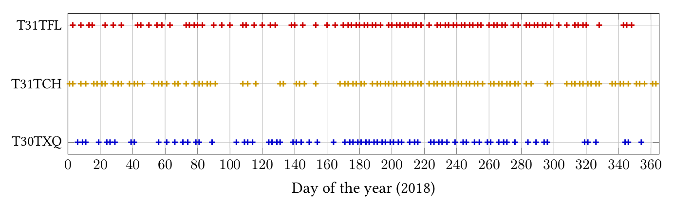
Secondly, not all the acquisitions in a swath contain the same dates. As such, the time series are irregularly sampled in the temporal domain: observations are not equally spaced in time due to the presence of clouds or cloud shadows. Indeed, if clouds are present in an image, the reflectance corresponds to the one of the clouds and not to the one of the land cover. Therefore, dates for which the image consists essentially of clouds (i.e. images containing more than 90% of clouds are not processed to the level 2A at THEIA) are removed. Figure 2 represents the temporal grids for three tiles (T30TXQ, T31TCH, T31TFL) and shows the misalingment phenomenon.

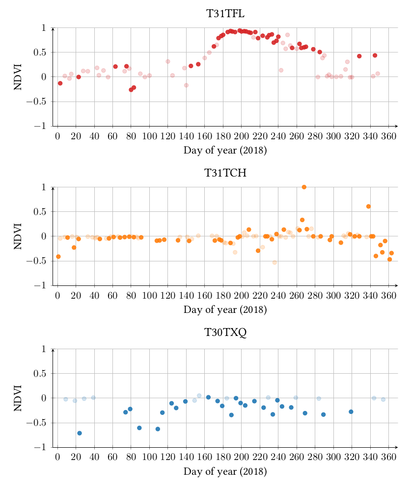
Finally, locally, different meteorological conditions, such as clouds, haze, mist or cloud shadow can cause technical artifacts for one pixel at a given date. This information is considered as corrupted and the pixel is declared as invalid. Therefore, the information at this date can be removed for this pixel leading to irregular temporal sampling. Therefore, the sampling of very close pixels may also be different. Figure 3 represents the NDVI profile for three pixels from these same tiles (T30TXQ, T31TCH, T31TFL). Both valid dates and cloudy / shadow dates are represented in this figure. A valid date corresponds to an acquired observation where no cloud or cloud shadow is detected by the level 2A processor. The pixel from the tile T31TFL has long periods without valid dates. The pixel from the tile T31TCH is the least impacted by the cloudy / shadow dates.

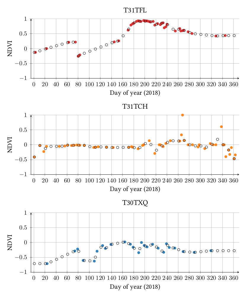
To cope with the clouds, cloud shadows and different temporal sampling betweem the tiles, the data can be linearly resampled onto a common set of virtual dates with an interval of ten days, for a total of 37 dates, as it is currently done in iota2. The first date corresponds to the day 1 of the year and the last day corresponds to the day 361 of the year. Figure 4 represents the linear interpolation for the three pixels described previously.

However, linear interpolation is performed independently of the classification task, i.e., the final task.  Li et al. [Li and Marlin, 2016] showed that an independent interpolation method directly followed by a classification method performed worse in terms of classification accuracy than methods trained end-to-end. Therefore, in the following, we propose to learn a representation optimized for the classification task.

Data set and experimental set up

The study area covers approximately 200 000 km2 in the south of metropolitan France and it is composed of 27 Sentinel-2 tiles, as displayed in Figure 1. All available acquisitions of level 2A between January and December 2018 were used (the preprocessing of the data is described more in detail in the paper) . Combining the five orbits, 303 unique acquisition dates are available.

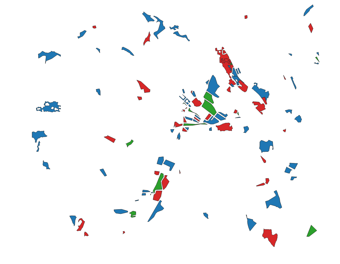
Pixels were randomly sampled from polygons over the full study area to create three spatially disjoint data subsets: training, validation and test, as illustrated in Figure 5. The polygons are disjoint between the three data sets. The three data sets are class-balanced: 4 000 pixels per class in the training data set, 1 000 pixels per class in the validation data set and 10 000 pixels per class in the test data set. Therefore, we have 92 000 pixels for the training data set, 23 000 pixels for the validation data test and 230 000 pixels for the test data set.

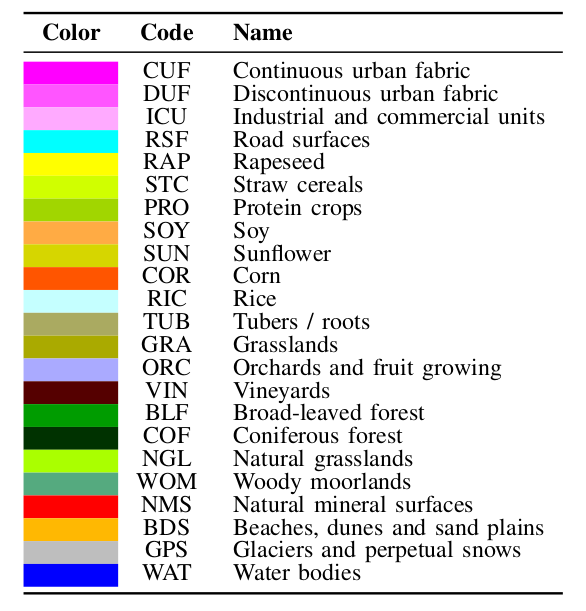
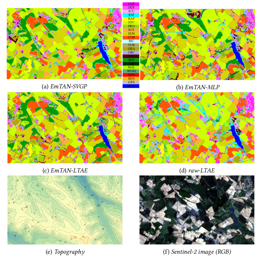
The reference data used in this work is composed of the 23 land cover classes from the OSO land cover map. The nomenclature and the color-code of the classes is given in Figure 6.

Method

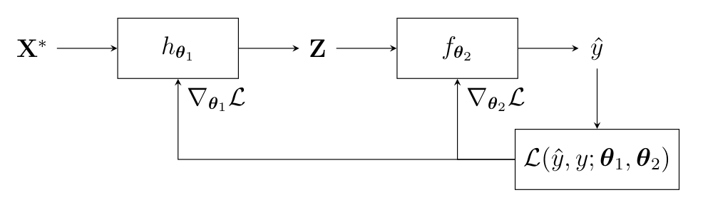
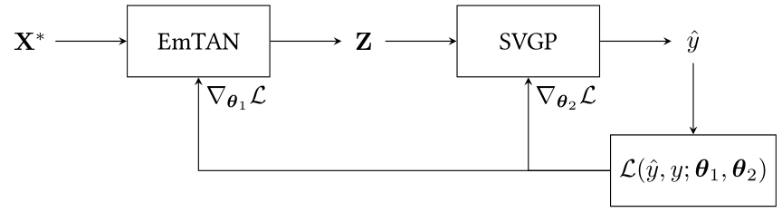
We propose to use end-to-end learning by combining a spatially informed interpolator called Extended multi Time Attention Networks (EmTAN) (first block) with a Stochastic Variational Gaussian Processes (SVGP) classifier, (second block), as illustrated in Figure 7. The model made of the EmTAN combined with the SVGP classifier is called EmTAN-SVGP.

Figure 7 represents the workflow for the classification of one irregular and unaligned pixel time series X* of size D × T through its learned latent representation Z of size D’ × R, with D the number of spectral features, T the total number of observations (in our case 303 unique acquisition dates), D’ the number of latent spectral (we take the liberty of using the term « spectral » as a misnomer, as it does not concern the temporal dimension) features and R the number of latent dates.

The EmTAN is a spatially informed interpolator as the spatial coordinates are integrated in the processing by means of spatial positional encoding. Besides, a spectro-temporal feature reduction is performed. Indeed, by taking R < T , the EmTAN allows to perform feature reduction in the temporal domain. Moreover, with D’ < D, a spectral reduction is performed. The spectro-temporal reduction allows to reduce the complexity of the SVGP classifier. The EmTAN is optimized by maximizing the classification accuracy, not the reconstruction error as it is conventionally done with standard interpolation methods. A more detailed description of the EmTAN and of the SVGP classifiers are provided in our articles: 10.1109/JSTARS.2023.3343921 and 10.1109/TGRS.2023.3234527.

Competitive methods

Four different classification methods are defined as competitive methods:

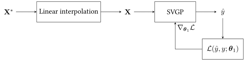
1. Gapfilled-SVGP: A SVGP classifier feeds with time series linearly interpolated every 10 days, as illustrated in Figure 8.

2. EmTAN-MLP: A Multi-layer Perceptron (MLP) classifier combined with the EmTAN, as illustrated in Figure 9.

3. EmTAN-LTAE: A Light Temporal Attention Encoder (LTAE) classifier combined with EmTAN, as illustrated in Figure 10.

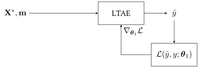
4. raw-LTAE: A LTAE classifier without EmTAN. Unlike SVGP or MLP classifiers, the LTAE classifier uses attention mechanisms. It may be redundant to use attention mechanisms both in the EmTAN and in the LTAE classifier. However, the LTAE classifier was not defined to deal with the irregular and unaligned time series pixels. Thus, we provide the mask m as an additional feature, as illustrated in Figure 11.

A more detailed description of these methods are provided in our article (10.1109/JSTARS.2023.3343921).

Results

Quantitative results

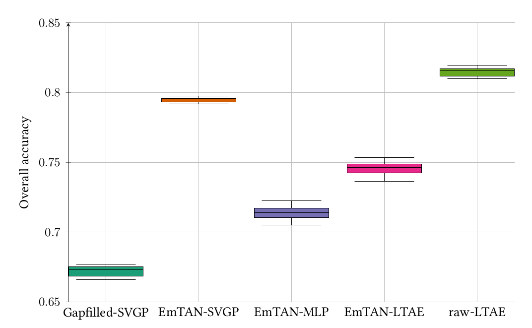
Figure 12 represents the overall accuracy (OA) for the five methods (Gapfilled-SVGP, EmTAN-SVGP, EmTAN-MLP, EmTAN-LTAE, raw-LTAE). For information, from previous works, we found that Gapfilled-SVGP is above the baseline, the Gapfilled-RF (Random Forest with linearly interpolated data every 10 days) from CES OSO (https://www.cesbio.cnrs.fr/multitemp/premieres-validations-de-la-carte-doccupation-du-sol-oso/). Therefore, these results are not represented in Figure 12.

The learned latent representation Z obtained by the EmTAN contains more meaningful information for the classification task for the SVGP classifier compared to the linearly interpolated data. Besides, the SVGP model took greater advantage of the interpolator than the MLP or the LTAE models. Indeed, the OA of the EmTAN-SVGP model is seven points above the EmTAN-MLP model and around four points above the EmTAN-LTAE model. Besides, the EmTAN-SVGP model is the model with the smallest dispersion. On the other hand, the EmTAN-SVGP model is in average two points below the raw-LTAE model. However, to compute the inference on a specific area (e.g. on a specific Sentinel-2 tile), the raw-LTAE requires the whole set of observed dates used during the training step (e.g. observed dates from all tiles) . This is not the case for our proposed model which is able to process pixels with a set of observed dates (e.g. the corresponding dates for one Sentinel-2 tile).  See our article (10.1109/JSTARS.2023.3343921) for more details.

Qualitative results

Figure 13 represents the land cover maps obtained for four methods (EmTAN-SVGP, EmTAN-MLP, EmTAN-LTAE, raw-LTAE) on a agricultural area around Toulouse. In the forest areas, it appears that the raw-LTAE model does not correctly predict the BLF class. In contrast, the predictions are homogeneous for the models using the EmTAN : EmTAN-SVGP, EmTAN-MLP and EmTAN-LTAE. For the mTANe-MLP and mTANe-LTAE models, the majority of the crops are surrounded by the class VIN whereas it would appear to be hedges instead. Finally, the results obtained for the EmTAN-SVGP, EmTAN-MLP and EmTAN-LTAE models showed that the main structures of the map are clearly represented (i.e. crop field borders). Therefore, these models provide the spatial information in the EmTAN without spatial over-smoothing.

Reconstruction

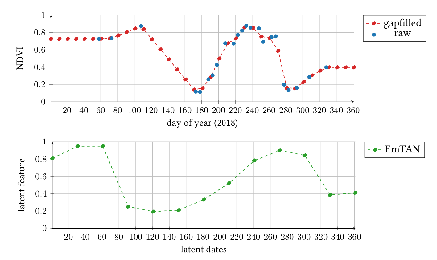
Figure 14 represents the comparison of three NDVI time series profiles from one pixel labeled as corn: the raw data, the linearly interpolated data and the learned latent representation obtained by the EmTAN. The latent representation Z clearly does not minimize the reconstruction error of the original time series. For instance, the second minimum of the NDVI observed around the day of the year 280 is not reconstructed. Yet, this is the representation that conducts to minimize the classification loss function of the SVGP. Besides, latent dates do not necessarily correspond to real dates, so time distortion can occur. The aim is to align the data in order to maximize classification performance.

Conclusion and perspectives

In this work, we have developed an end-to-end model that combines a time and space informed kernel interpolator (EmTAN) with the SVGP classifier. We were able to process irregular and unaligned SITS without any temporal re-sampling preprocessing. This method outperformed the simple SVGP classifier with linearly preprocessed interpolated data. Therefore, from previous works, it also outperformed the CES OSO based approach (RF classifier with linearly preprocessed interpolated data and spatial stratification) in our study area. A perspective could be to apply the model over all metropolitan France, as it is done for OSO and to compare with the CES OSO based approach.

Another perspective could be to use pluriannual time series instead of a one-year time series (i.e. multitemporal data fusion). The EmTAN could learn periodic patterns over the years. Besides, another perspective could be to combine multi-modal time series. Adding a radar sensor (i.e. Sentinel-1) or other type of optical sensors (i.e. Landsat 8 with its thermal bands) could improve the representation for the classification task. The ability of the EmTAN to process unaligned time series would make the fusion of multi-sensor data straightforward.

Acknowledgements

This post was written by Valentine Bellet during her PhD in CESBIO. Valentine is now at CNES.

Our warmest thanks go to Benjamin Tardy, from CS Group – France, for his support and help during the generation of the different data sets and the production of land cover classification maps with the iota2 software. We would also like to thank CNES for the provision of its high performance computing (HPC) infrastructure to run the experiments presented in this paper and the associated help.

This work was supported by the Natural Intelligence Toulouse Institute (ANITI) from Université Fédérale Toulouse Midi-Pyrénées under grant agreement ANITI ANR-19-PI3A-0004 (this PhD is co-founded by CS-Group and by Centre National d’Études Spatiales (CNES)).