Iota2 can also do regression
Iota2 is constantly evolving, as you can check at the gitlab repository. Bugs fix, documentation updates and dependency version upgrade are done regularly. Also, new features are introduced such as the support of Landsat 8 & 9 images, including thermal images, or for what concerns us in this post, the support of regression models.
In machine learning, regression algorithms are supervised methods1 used to estimate a continuous variable from some observations (see more here: https://en.wikipedia.org/wiki/Regression_analysis). In remote sensing, regression is used to recover biophysical or agronomic variables from satellite images. For instance, it is used in SNAP (https://step.esa.int/main/download/snap-download/) to estimate LAI from Sentinel-2 surface reflectance.
At the beginning, iota2 was designed to perform classification (estimation of categorical values) whose framework shares a lot with regression but has also some significant differences. To cite the main ones: the loss function as well as how the data are split differ between classification and regression. Some other differences may exist depending on the algorithm. Fortunately, since the end of 2023, iota2 is also able to perform regression with satellite image time series.
In this post, we are going to illustrate the workflow of the regression builder on a simple case: estimate the red band value of one Sentinel-2 date having observed other Sentinel-2 dates. Full information can be found in the online documentation: https://docs.iota2.net/develop/i2_regression_tutorial.html.
1. Iota2 configuration
1.1. Data set
To illustrate iota2 capability, we set-up the following data set: One year of Sentinel2 data over the tile T31TCJ, starting on the 2018-02-10 until the 2018-12-10, from which we try to infer the red band of 2018-12-17. Yes, it is not a real problem but since Sentinel2 data are free and open-source, we can put online this toy data to let you reproduce the simulation: https://zenodo.org/records/10574545.
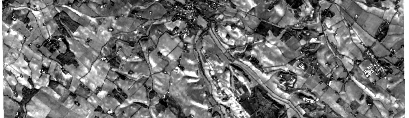
The area in pixel size is 909*807, see figure below. We have randomly extracted pixel values from the red band for training and validation and put everything in a shapefile.

Figure 1: Area of interest (background image © OpenStreetMap contributors)
1.2. Configuration file
As usual with iota2, the configuration file contains all the necessary information and it is very similar to what is required for classification (see https://www.cesbio.cnrs.fr/multitemp/iota2-latest-release-deep-learning-at-the-menu for a more detailed discussion on the configuration file). We use the following one
chain:
{
    s2_path: "<<path_dir>>/src/sensor_data"
    output_path: "<<path_dir>>/Iota2Outputs/"
    remove_output_path: True
    list_tile: "T31TCJ"
    ground_truth: "<<path_dir>>/src/vector_data/ref_small.shp"
    data_field: "code"
    spatial_resolution: 10
    proj: "EPSG:2154"
    first_step: "init"
    last_step: "validation"
}

arg_train:
{
    runs: 1
    ratio : 0.75
    sample_selection:
    {
        "sampler": "periodic",
        "strategy": "all",
    }
}
scikit_models_parameters:
{
    model_type:"RandomForestRegressor"
    keyword_arguments:
    {
        n_estimators : 200
        n_jobs : -1
    }
}
python_data_managing:
{
    number_of_chunks: 10
}
builders:
{
    builders_class_name: ["i2_regression"]
}
sentinel_2:
{
    temporal_resolution:10
}
1.3. Results
146,579 pixels were used to train the random forest with 200 trees, and 48,860 pixels were used as test samples to compute the prediction accuracy. Iota2 returns the following accuracy results for the test set (we normalize the data to have reflectance and not digital number):
| max error | mean absolute error | mean squared error | median absolute error | r2 score |
|---|---|---|---|---|
| 0.200 | 0.005 | 6.383e-5 | 0.003 | 0.894 |
Well, the results are good 🙂 Given one year of data, it is possible to infer most of the pixel values 7 days later. Congrats iota2 !
If we look at the map, we can see that most of the errors are made over areas with light clouds. It would have been the case also for areas with rapid changes since we have done nothing particular to deal with changes in the regression set-up. Figures below show the true red band, the estimated one and the prediction error, computed as the normalized absolute error.
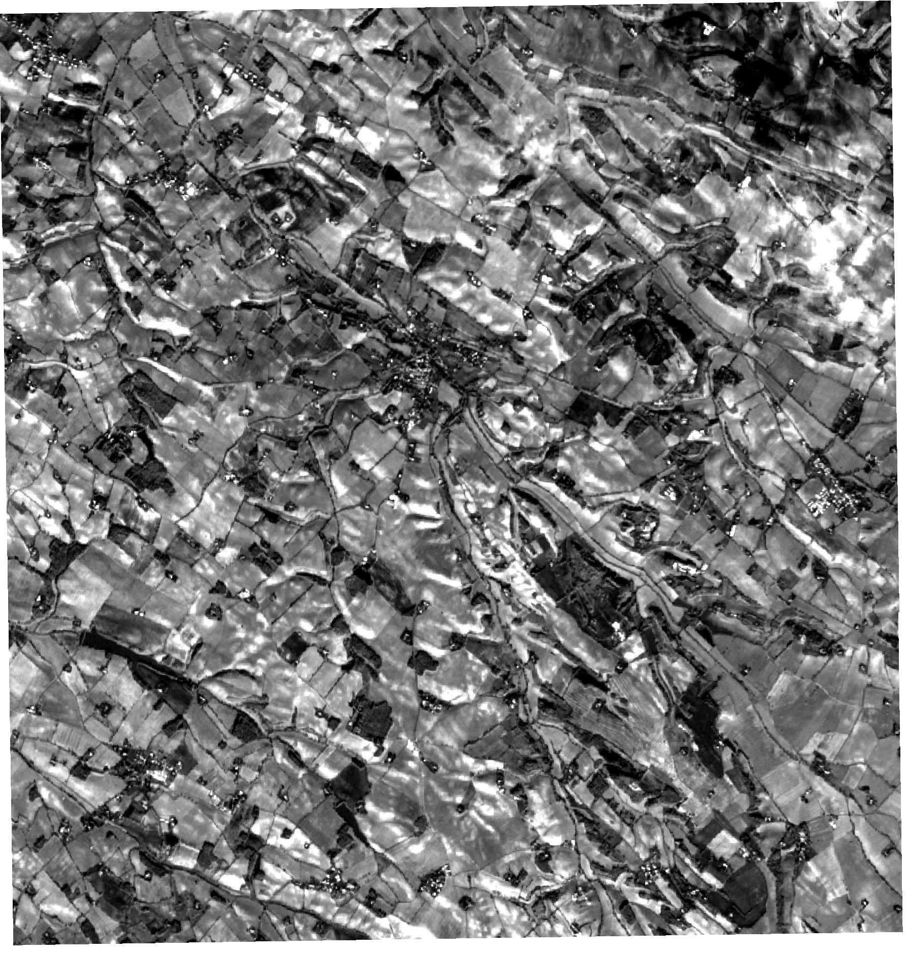
Figure 2: True Sentinel-2 red band.
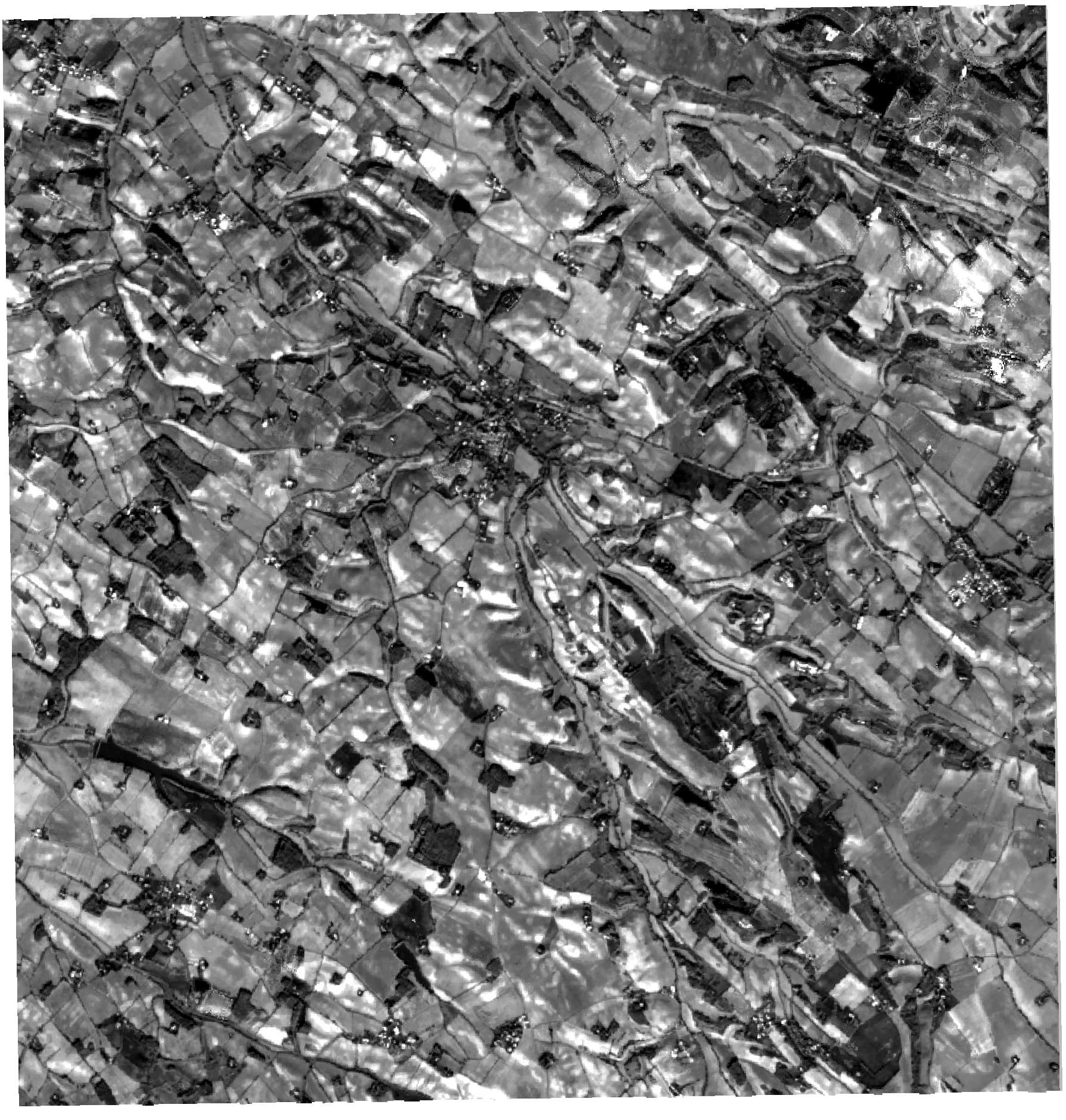
Figure 3: Predicted Sentinel-2 red band.
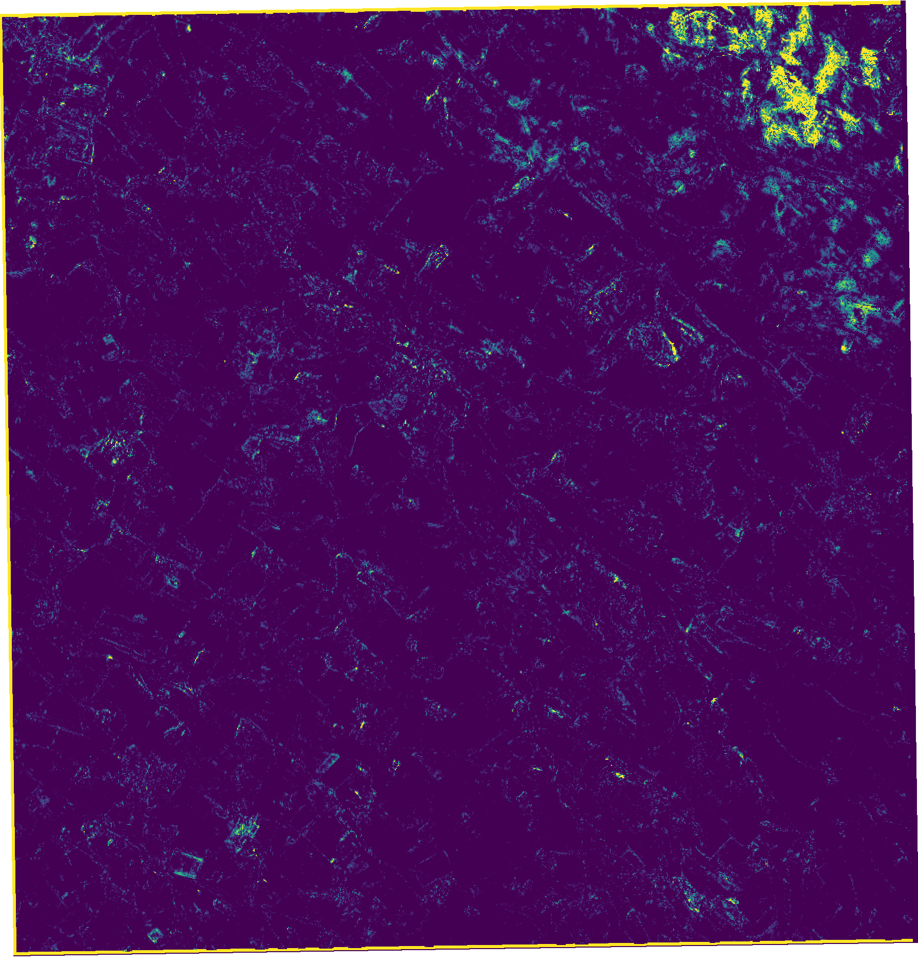
Figure 4: Prediction error in percentage; \(\frac{|true-pred|}{true}\).
2. Discussion
Iota2 offers many more possibilties, as for the classification framework: multi-run, data augmentation or spatial stratification for instance. The online documentation (https://docs.iota2.net/develop/i2_regression_tutorial.html) provides all the relevant information: please check it if needed.
In this short post, we have used random forest, but other methods are available, in particular deep learning based methods. For now, it is possible to regress only one parameter at time. A possible extension would be to regress several variables simultaneously.
This new feature has been used to map moving date of permanent grasslands at the national scale for year 2022. This work is in progress, but you can see current results on zenodo (draft map: https://zenodo.org/records/10118125). Iota2 has simplified greatly the production of such large scale map.
3. Acknowledgement
Iota2 development team is composed of Arthur Vincent and Benjamin Tardy, from CS Group. Hugo Trentesaux spent 10 months (October 2021 – July 2022) in the team and started the development of the regression. Then, Hélène Touchais continued the IT developments since November 2022 and has concluded this work at the end of 2023.
Developments are coordinated by Jordi Inglada, CNES & CESBIO-lab. Promotion and training are ensured by Mathieu Fauvel, INRAe & CESBIO-lab and Vincent Thierion, INRAe & CESBIO-lab.
The development was funded by several projects: CNES-PARCELLE, CNES-SWOT Aval, ANR-MAESTRIA and ANR-3IA-ANITI with the support of CESBIO-lab and Theia Data Center. Iota2 has a steering committee which is described here.
We thank the Theia Data Center for making the Sentinel-2 time series available and ready to use.
Footnotes:
Need some ground truth.