Iota2 latest release – Deep Learning at the menu
Table of Contents
1. New iota2 release
The last version of iota2 (https://framagit.org/iota2-project/iota2) released on includes many new features. A complete list of changes is available here. Among them, let cite a few that may be of interest for users:
External features with padding: External features is a iota2 feature that allows to include user-defined computation (e.g. spectral indices) in the processing chain. They come now with a padding option. Each chunk can have an overlap with all his adjacent chunks and therefore it is possible to perform basic spatial processing with external features without discontinuity issues. Check this for a toy example.
issue: https://framagit.org/iota2-project/iota2/-/issues/466
doc: https://docs.iota2.net/develop/external_features.htmlExternal features with parameters: The function provided by the user can now have their parameters set directly in the configuration file. It is no longer necessary to hard-coded them in the python file.
issue: https://framagit.org/iota2-project/iota2/-/issues/393
doc: https://docs.iota2.net/develop/external_features.html#examples- Documentation: The documentation is now hosted at https://docs.iota2.net/master/. An open access labwork is also available https://docs.iota2.net/training/labworks.html for advanced users that have already done the tutorial from the documentation.
Deep Learning workflow: iota2 is now able to perform classification with (deep) neural networks. It is possible to use either one of the pre-defined network architectures provided in iota2 or to define its own architecture. The workflow is based on the library Pytorch.
issue: https://framagit.org/iota2-project/iota2/-/issues/194
doc: https://docs.iota2.net/develop/deep_learning.html
Introducing the deeplearning workflow was a hard job: including all the machinery for batches training as well as various neural architectures in the workflow has introduced some major internal changes in iota2. A lot of work were done to ensure iota2 is able to scale well accordingly the size of the data to be classified when deep learning is used. In the following, we will provide an example of classification of large scale Sentinel 2 time series using deep learning.
2. Classification using deep learning
In this post we discuss about deep learning in iota2. We describe the data set used for the experiment, the different pre-processing done to prepare the different training/validation files, the deep neural network used and how it is learned with iota2. Then classification results (classification accuracy as well as classification maps) will be presented to enlight the capacity of iota2 to easily perform large scale analysis, run various experiments and compare their outputs.
2.1. Material
2.1.1. Satellite image time series
For the experiments, we use all the Level-2A acquisitions available from Theia Data Center (https://www.theia-land.fr/en/products/) for one year (2018) over 4 Sentinel 2 tiles ([“31TCJ”, “31TCK”, “31TDJ”, “31TDK”]). See figure 1. The raw files size amount to 777 Gigabytes.
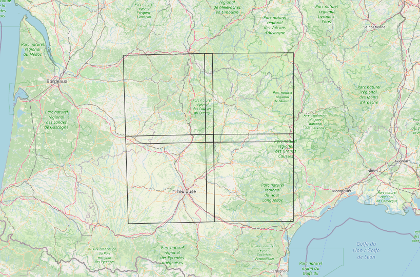
Figure 1: Sentinel 2 tiles used in the experiments (background map © OpenStreetMap contributors).
2.1.2. Preparation of the ground truth data
For the ground truth, we have extracted the data from the database used to produce the OSO product (https://www.theia-land.fr/en/ceslist/land-cover-sec/). The database was constructed by merging several open source databases, such as Corine Land Cover. The whole process is described in (Inglada et al. 2017). The 23-categories nomenclature is detailed here: https://www.theia-land.fr/en/product/land-cover-map/. An overview is given figure 2.
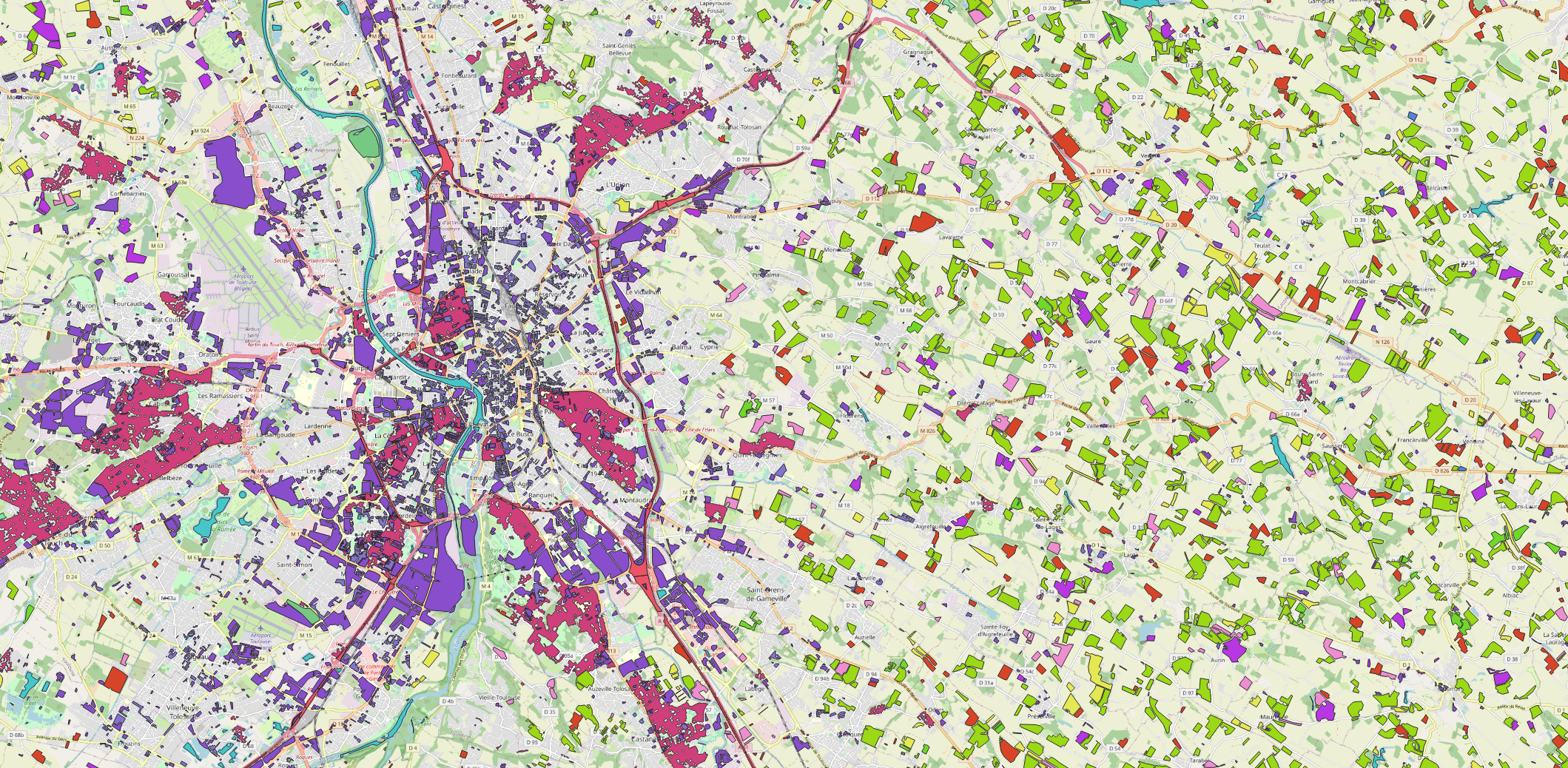
Figure 2: Zoom of the ground truth over the city of Toulouse. Each colored polygon corresponds to a labelized area (background map © OpenStreetMap contributors).
2.1.2.1. Sub data set
This step is not mandatory and is used here only for illustrative purpose.
In order to run several classifications and to assess quantitatively and qualitatively the capacity of deep learning model, 4 sub-data set were build using a leave-one-tile-out procedure: training samples for 3 tiles will be used to train the model and samples for the remaining tile will be left out for testing. The process will be repeated for each subset of 3 tiles from a set of 4 tiles (i.e. 4 times !). We will see later how iota2 allows to perform several classifications tasks from different ground truth data easily.
For now, once you have a vector file containing your tiles and the (big) database, running this kind of code
should do the job (at least for us it does!): construct 4 couples of training/testing vector files. You can adapt it to your own configuration. An example of one sub data set is given figure 3.
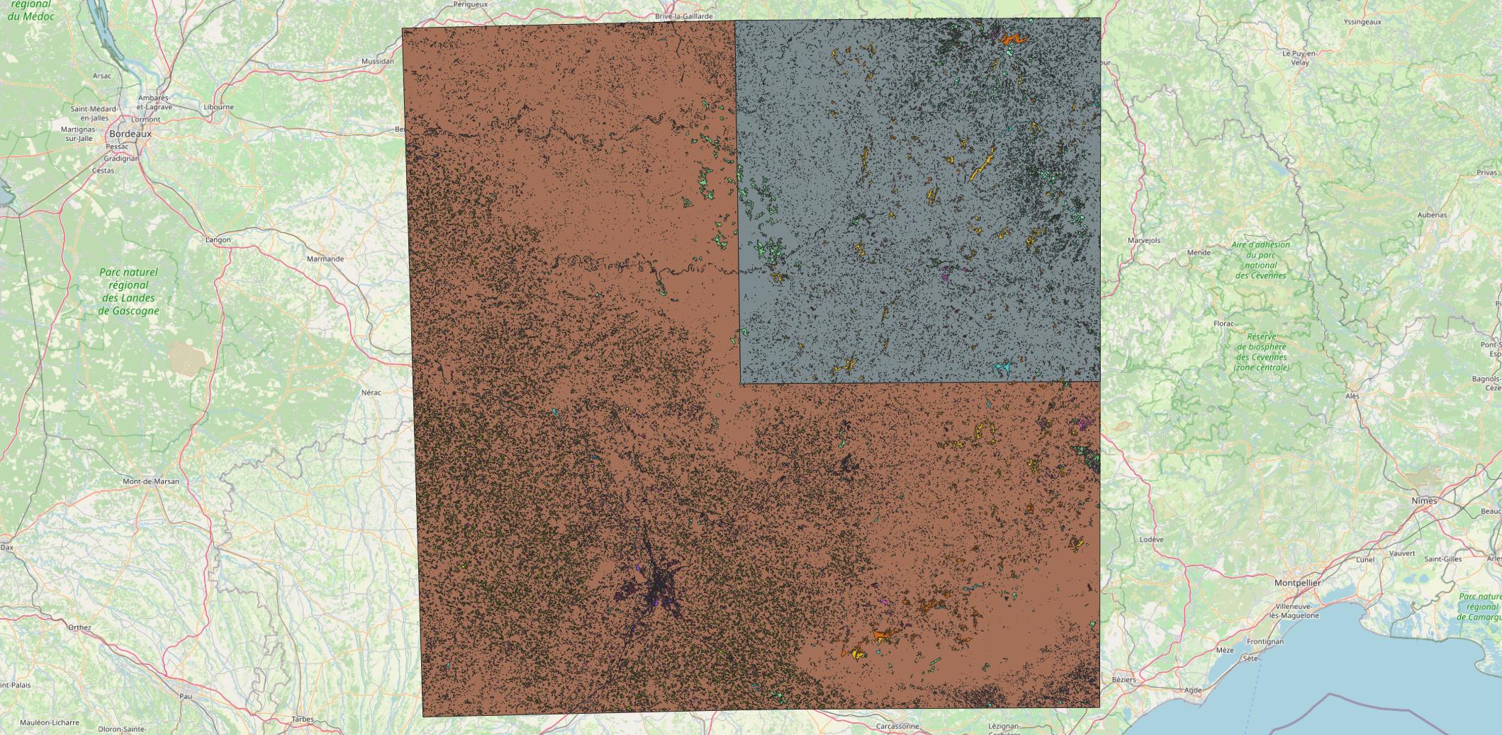
Figure 3: Sub data set: polygons from the brown area are used to train the model and polygons from the gray area are used to test the model. There are 4 different configurations, one for each tile left-out. (background map © OpenStreetMap contributors).
2.1.2.2. Clean the ground truth vector file
The final step in the ground truth data preparation is to clean the ground truth file: when manipulating vector files it is common to have multi-polygons, empty or duplicate geometries. Such problematic features should be handled before running iota2. Fortunately, iota2 is packed with the necessary tools (check_database.py, available from the iota2 conda environment) to prevent all these annoying things that happen when you process large vector files. The code snippet in 1 shows how to run the tool on the ground truth file.
for i in 0 1 2 3
do
    check_database.py \
        -in.vector ../data/gt_${i}.shp \
        -out.vector ../data/gt_${i}_clean.shp \
        -dataField code -epsg 2154 \
        -doCorrections True
done
2.2. Configuration of iota2
This part is mainly based on the documentation (https://docs.iota2.net/develop/deep_learning.html) as well as a tutorial we gave (https://docs.iota2.net/training/labworks.html). We encourage the interested reader to carefully reads these links for a deeper (!) understanding.
2.2.1. Config and ressources files
As usual with iota2, the first step is to set-up the configuration file. This file hosts most of the information required to run the computation (where are the data, the reference file, the output folder etc …). The following link is a good start to understand the configuration file: https://docs.iota2.net/develop/i2_classification_tutorial.html#understand-the-configuration-file. We try to make the following understandable without the need to fully read it.
To compute the classification accuracy obtained on the area covered by ground truth used for training, we indicate to iota2 to split polygons from the ground truth file into two files, one for training and one for testing with a ratio of 75%:
split_ground_truth : True
ratio : 0.75
It means that 75% of the available polygons for each class is used for training while the remaining is used for testing. Note that we do not talk about pixels here. By splitting at the polygons level, we ensure that pixels from a polygon are used either for training or testing. This is a way to reduce the spatial auto-correlation effect between pixels when assessing the classification accuracy.
We need now to set-up how training pixels are selected from the polygons. Iota2 relies on OTB sampling tools (https://www.orfeo-toolbox.org/CookBook/Applications/app_SampleSelection.html). For this experiment, we asked for a maximum number of pixels of 100000 with a periodic sampler.
arg_train :
{
    sample_selection :
  {
        "sampler" : "periodic"
        "strategy": "constant"
        "strategy.constant.nb" : 100000
  }

}
We are working on 4 different tiles, each of them having its own temporal sampling. Furthermore, we need to deals with clouds issues (Hagolle et al. 2010). Iota2 uses temporal gap-filling as discussed in (Inglada et al. 2015). In this work, we use a temporal step-size of 10 days, i.e., we have 37 dates. Iota2 also computes per default three indices (NDVI, NDWI and Brightness). Hence, for a each pixel we have a set of 481 features (37\(\times\)13).
For the deep neural network, we use the default implementation in iota2. However, it is possible to define its own architecture (https://docs.iota2.net/develop/deep_learning.html?highlight=deep%20learning#desc-dl-module). In our case, the network is composed of four layers (see Table 1) with a relu function between each of them (https://framagit.org/iota2-project/iota2/-/blob/develop/iota2/learning/pytorch/torch_nn_bank.py#L276).
| Input size | Output size | |
| First Layer | 481 | 240 |
| Second Layer | 240 | 69 |
| Third Layer | 69 | 69 |
| Last Layer | 69 | 23 |
ADAM solver was used for the optimization, with a learningrate of \(10^{-5}\) and a batch size of 4096. 200 epochs were performed and a validation sample set, extracted from the training pixels is used to monitor the optimization. The best model in terms of Fscore is selected. Off course all these options are configurable with iota2. A full configuration file is given in Listing 2.
chain :
{
  output_path : "/datalocal1/share/fauvelm/blog_post_iota2_output/outputs_3"
  remove_output_path : True
  check_inputs : True
  list_tile : "T31TCJ T31TDJ T31TCK T31TDK"
  data_field : "code"
  s2_path : "/datalocal1/share/PARCELLE/S2/"
  ground_truth : "/home/fauvelm/BlogPostIota2/data/gt_3_clean.shp"

  spatial_resolution : 10
  color_table : "/home/fauvelm/BlogPostIota2/data/colorFile.txt"
  nomenclature_path : "/home/fauvelm/BlogPostIota2/data/nomenclature.txt"
  first_step : 'init'
  last_step : 'validation'
  proj : "EPSG:2154"
  split_ground_truth : True
  ratio : 0.75
}

arg_train :
{
  runs : 1
  random_seed : 0
  sample_selection :
  {
        "sampler" : "periodic"
        "strategy": "constant"
        "strategy.constant.nb" : 100000
  }
  deep_learning_parameters :
  {
        dl_name : "MLPClassifier"
        epochs : 200
        model_selection_criterion : "fscore"
        num_workers : 12
        hyperparameters_solver : {
                        "batch_size" : [4096],
                        "learning_rate" : [0.00001]
                        }
    }
}

arg_classification :
{
        enable_probability_map : True
}

python_data_managing :
{
        number_of_chunks : 50
}

sentinel_2 :
{
        temporal_resolution : 10
}

task_retry_limits :
{
         allowed_retry : 0
         maximum_ram : 180.0
         maximum_cpu : 40
}
The configuration file is now ready and the chain can be launched, as described in the documentation. Classification accuracy will be outputted in the directory final as well as the final classification map and related iota2 outputs.
2.2.2. Iteration over the different sub ground truth files
However, in this post we want to go a bit further to enlighten how easy it is to run several simulations with iota2. As discussed in 2.1.2.1, we have generated a set of pair of spatially disjoint ground truth vector files for training and for testing. Also, remind that iota2 starts by splitting the provided training ground truth file into two spatially disjoints files, one used to train the model and the other used to test the model. In such particular configuration, we have now two test files:
- One extracted from the same area than the training samples,
- One extracted from a different area than the training samples.
With this files, we can do a spatial cross validation estimation of the classification accuracy, as discussed in (Ploton et al. 2020). To perform such analysis, we first stop the chain after the prediction of the classification map (setting the parameter as last_step : 'mosaic') and we manually add another step to estimate the confusion matrix from both sets. We rely on the OTB tools: https://www.orfeo-toolbox.org/CookBook/Applications/app_ComputeConfusionMatrix.html?highlight=confusion%20matrix.
The last ingredient is to be able to loop over the different tiles configurations, i.e., to iterate over the cross-validation folds. This is where iota2 is really powerful: we just need to change few parameters in the configuration file to run all the different experiments. In this case, we have to change the ground truth filenames and the output directory. To make it simple, we indexed our simulations from 0 to 3 and use sed shell tool to modify the configuration file in the big loop:
sed -i "s/outputs_\([0-9]\)/outputs_${REGION}/" /home/fauvelm/BlogPostIota2/configs/config_base.cfg
sed -i "s/gt_\([0-9]\)_clean/gt_${REGION}_clean/" /home/fauvelm/BlogPostIota2/configs/config_base.cfg
The global script is given in Listing 3.
#/user/bin/bash

# Set ulmit
ulimit -u 6000

# Set conda env
source ~/.source_conda
conda activate iota2-env

# Loop over region
for REGION in 0 1 2 3
do
    echo Processing Region ${REGION}
    # (Delate and) Create output repertory
    OUTDIR=/datalocal1/share/fauvelm/blog_post_iota2_output/outputs_${REGION}/
    if [ -d "${OUTDIR}" ]; then rm -Rf ${OUTDIR}; fi
    mkdir ${OUTDIR}

    # Update config file
    sed -i "s/outputs_\([0-9]\)/outputs_${REGION}/" /home/fauvelm/BlogPostIota2/configs/config_base.cfg
    sed -i "s/gt_\([0-9]\)_clean/gt_${REGION}_clean/" /home/fauvelm/BlogPostIota2/configs/config_base.cfg

    # Run iota2
    Iota2.py \
        -config /home/fauvelm/BlogPostIota2/configs/config_base.cfg \
        -config_ressources /home/fauvelm/BlogPostIota2/configs/ressources.cfg \
        -scheduler_type localCluster \
        -nb_parallel_tasks 2


    # Compute Confusion Matrix for test samples
    otbcli_ComputeConfusionMatrix \
        -in ${OUTDIR}final/Classif_Seed_0.tif \
        -out ${OUTDIR}confu_test.txt \
        -format confusionmatrix \
        -ref vector -ref.vector.in /home/fauvelm/BlogPostIota2/data/tgt_0.shp \
        -ref.vector.field code \
        -ram 16384

    # Merge validation samples
    ogrmerge.py -f SQLITE -o ${OUTDIR}merged_val.sqlite \
                ${OUTDIR}dataAppVal/*_val.sqlite


    # Compute Confusion Matrix for train samples
    otbcli_ComputeConfusionMatrix \
        -in ${OUTDIR}final/Classif_Seed_0.tif \
        -out ${OUTDIR}confu_train.txt \
        -format confusionmatrix \
        -ref vector -ref.vector.in ${OUTDIR}merged_val.sqlite \
        -ref.vector.field code \
        -ram 16384
done

python compute_accuracy.py
Then we can compute classification metrics, such as the overall accuracy, the Kappa coefficient and the average Fscore. For this post, we have written a short python script to perform such operations: https://gitlab.cesbio.omp.eu/fauvelm/multitempblogspot/-/blob/main/scripts/compute_accuracy.py.
We can just run it, using nohup for instance, take a coffee, a slice of cheesecake and wait for the results 🙂
2.3. Results
Results provided by iota2 will be discussed in this section. The idea is not to perform a full analysis, but to glance through the possibilities offer by iota2. The simulations were run on computer with 48 Intel(R) Xeon(R) Gold 6136 CPU @ 3.00GHz, 188 Gb of RAM and a NVIDIA GV100GL [Tesla V100 PCIe 32GB].
2.4. Numerical results
First we can check the actual number of training samples used to train the model. Iota2 provides the total number of training samples used (https://docs.iota2.net/develop/iota2_samples_management.html?highlight=class_statistics%20csv#tracing-back-the-actual-number-of-samples). Table 2 provides the number of training samples extracted to learn the MLP. Yes, you read it well 1.8 millions of samples for only 4 tiles. During training, 80% of the samples were used to optimized the model and 20% were used to validate and monitor the model after each epoch. Four metrics were computed automatically by iota2 to monitor the optimization: the cross-entropy (same loss that is used to optimize the network), the overall accuracy, the Kappa coefficient and the F-score. Figures 4 and 5 display the evolution of the different metrics along the epochs. The model used for the classification is the one with the highest F-score.
| Class Name | Label | Total |
|---|---|---|
| Continuous urban fabric | 1 | 67899 |
| Discontinuous urban fabric | 2 | 100000 |
| Industrial and commercial units | 3 | 100000 |
| Road surfaces | 4 | 47664 |
| Rapeseed | 5 | 100000 |
| Straw cereals | 6 | 100000 |
| Protein crops | 7 | 100000 |
| Soy | 8 | 100000 |
| Sunflower | 9 | 100000 |
| Corn | 10 | 100000 |
| Rice | 11 | 0 |
| Tubers / roots | 12 | 53094 |
| Grasslands | 13 | 100000 |
| Orchards | 14 | 100000 |
| Vineyards | 15 | 100000 |
| Broad-leaved forest | 16 | 100000 |
| Coniferous forest | 17 | 100000 |
| Natural grasslands | 18 | 100000 |
| Woody moorlands | 19 | 100000 |
| Natural mineral surfaces | 20 | 11675 |
| Beaches, dunes and sand plains | 21 | 0 |
| Glaciers and perpetual snows | 22 | 0 |
| Water Bodies | 23 | 100000 |
| Others | 255 | 0 |
| Total | 1780332 |

Figure 4: Loss function on the training and validation set.
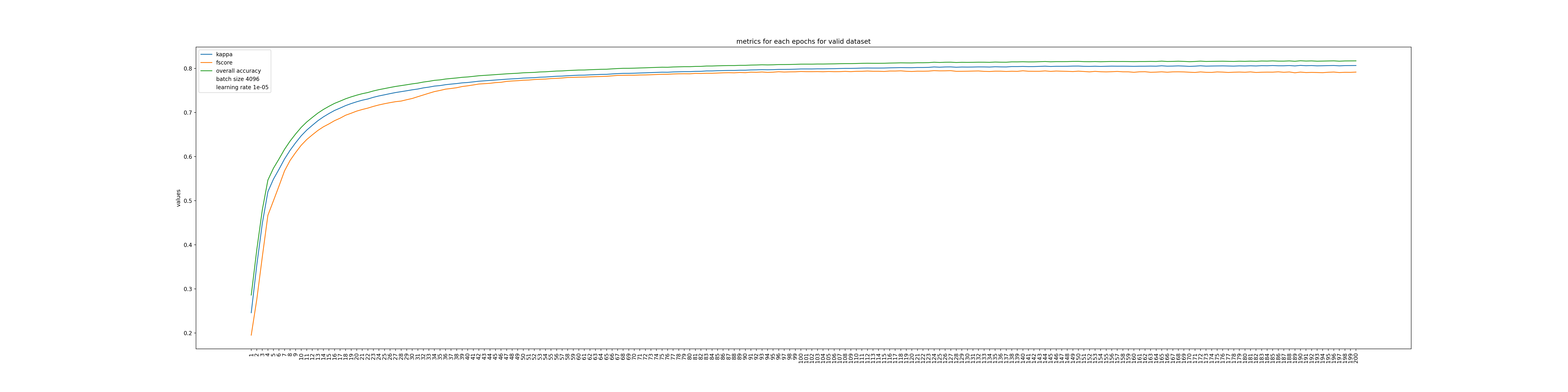
Figure 5: Classification metrics computed in the validation set.
For this set-up, the overall accuracy, the Kappa coefficient and the average F1 score are 0.85, 0.83 and 0.73, respectively. Which is in line with others results over the same area (Inglada et al. 2017).
Classification metrics provide quantitative assessment of the classification map. But it is still useful to do a qualitative analysis of the maps, especially at large scale where phenology, topography and others factors can influence drastically the reflectance signal. Off course, Iota2 allows to output the classification maps ! We choose three different sites, display on figures 6, 7 and 8. The full classification map is available here.
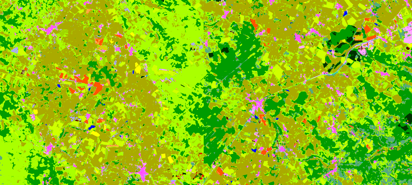
Figure 6: Classification map for an area located between two tiles.
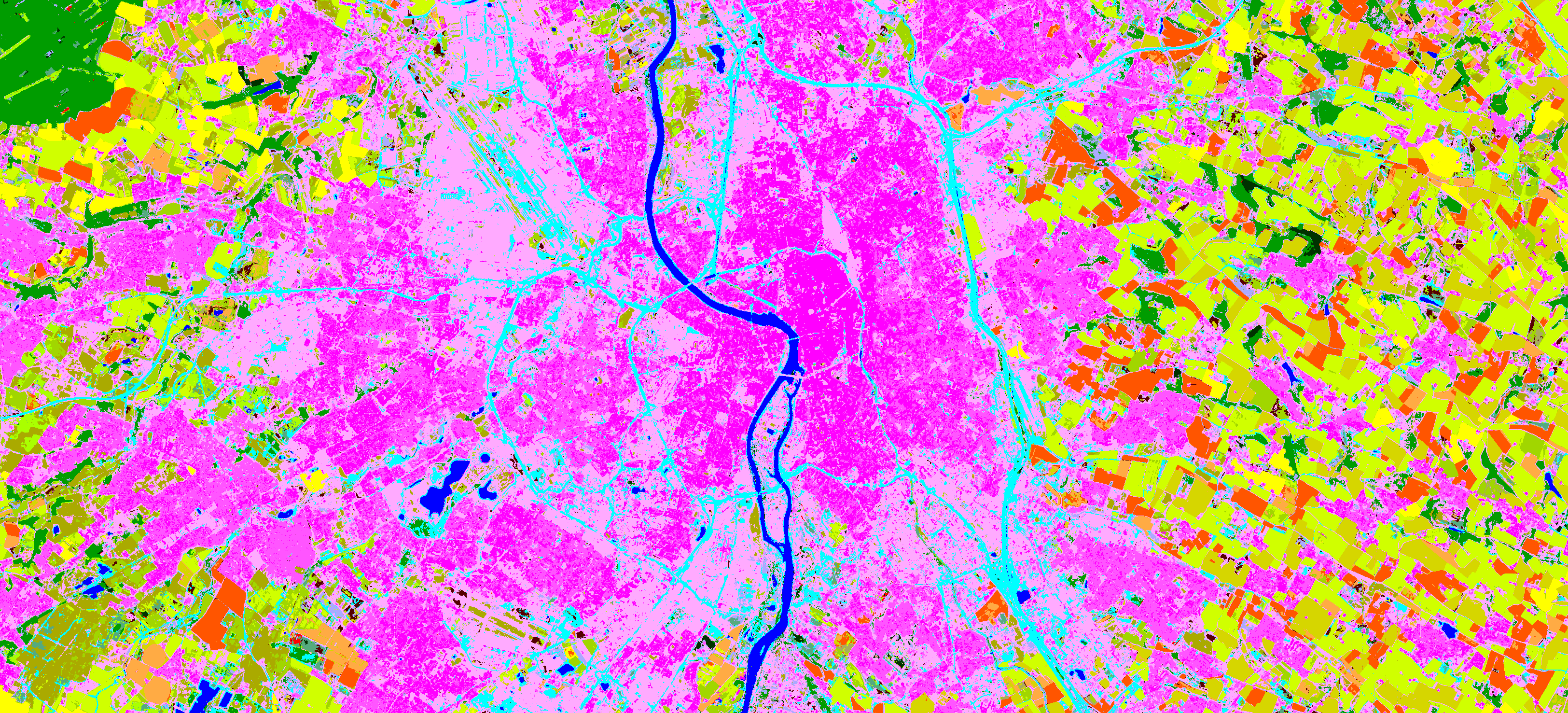
Figure 7: Classification map for an area over the city of Toulouse.
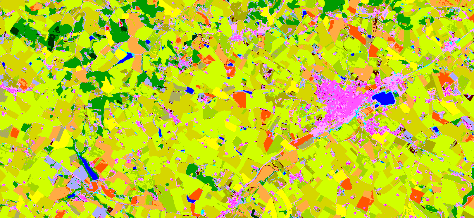
Figure 8: Classification map for a crop land area.
2.4.1. Results for the different sub ground truth files
The figure 9 shows the Fscore for the 4 models (coming from the 4 different runs), and the 2 test sets. We can easily see that depending on the tile left out, the difference of classification accuracy in terms of Fscore between test samples extracted from the same or disjoint area can be significant. Discussing the reasons why the performance are decreasing and what metrics should we use to asses the map accuracy are out of the scope of this post. It is indeed a controversy topic in remote sensing (Wadoux et al. 2021). We just want to emphasize that iota2 simplifies and automatizes a lot the process of validation, especially at large scale. Using this spatial cross validation with 4 folds, the mean estimated Fscore is 0.59 with a standard deviation of 0.08, which is indeed much lower than the 0.73 estimated in the previous part.
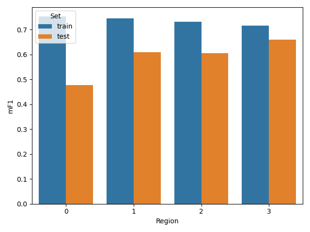
Figure 9: Fscore computed on samples from the same tiles used for training (train) and from one tile left out from the training region (test).
The different classification maps are displayed in the animated figures 10, 11 and 12. The first one displays a tricky situation at a frontier of two tiles. We can see a strong discontinuity, whatever the model used. For the second case over Toulouse, there is a global agreement between the 4 models, except for the class Continuous Urban Fabric (pink) that disappears for one model: the one learnt without data coming from the tile containing Toulouse (T31TCJ). The last area exhibits a global agreement with some slight disagreements for some crops. Note, the objective is not to fuse/combine the different results, but rather to quantitatively observed the differences in terms of classification maps when the ground truth is changed.
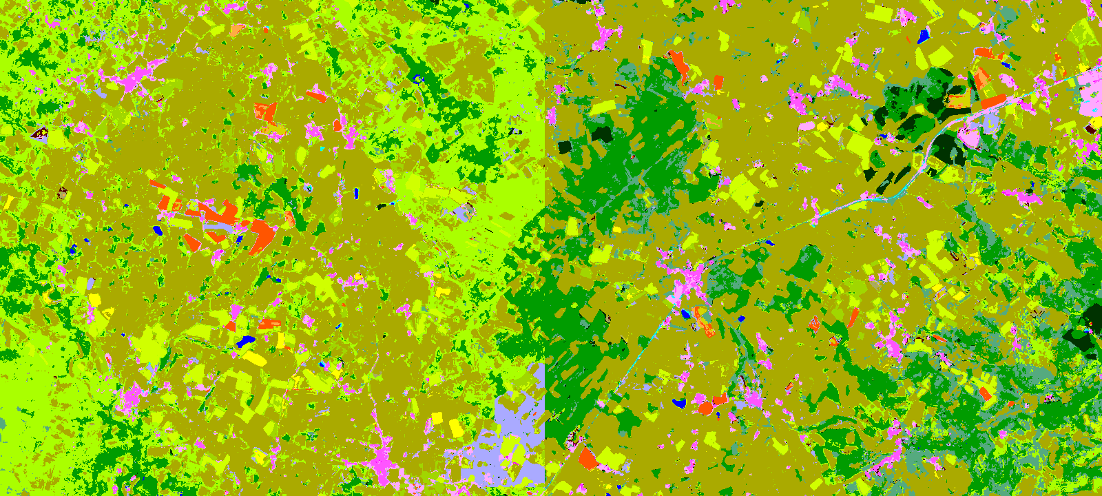
Figure 10: Classification maps for the 4 runs for an area located between two tiles.
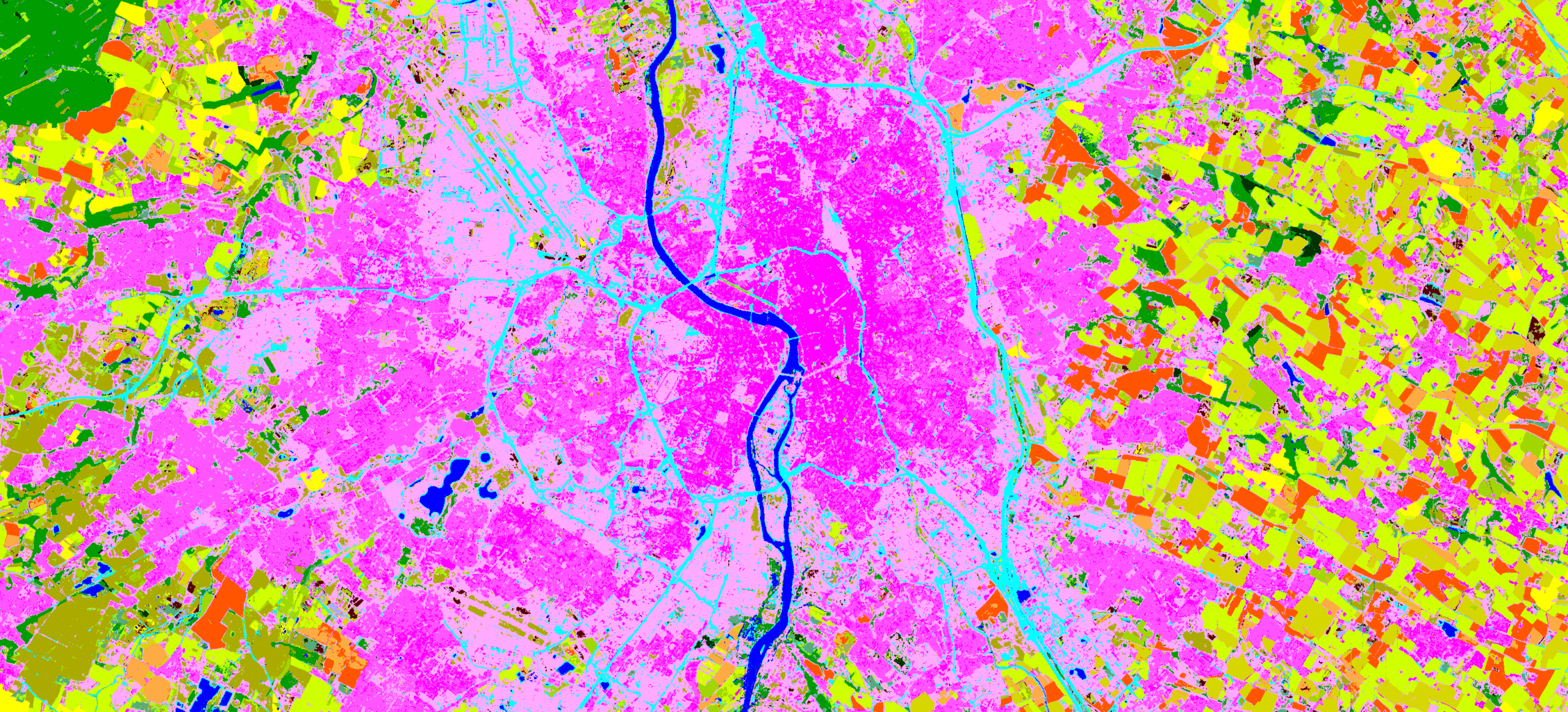
Figure 11: Classification maps for the 4 runs over the city of Toulouse.
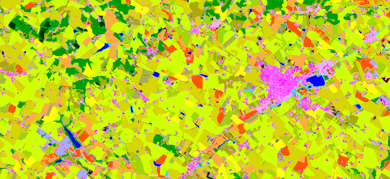
Figure 12: Classification maps for the 4 runs for a crop land area.
A finer analysis could be done, indeed. But we let this as an homework for interested reader: all the materials for the simulation are available here
and the Level-2A MAJA processed Sentinel-2 data are downloadable from Theia Data Center (try this out: https://github.com/olivierhagolle/Sentinel-download), while the ground truth data can be downloaded here.
3. Conclusions
To conclude, in this post we have presented briefly the latest release of iota2. Then, we focused on the deep learning classification workflow to classify 4 tiles of one year of Sentinel-2 time series. Even if it was only four tiles, it amount to process around 800 Gb of data, and with our data set, about \(4\times10^{7}\) pixels to be classified. We have skipped a lot of parts of the worklow, that iota2 takes care (projection, upsampling, gapfilling, streaming, multiple run, mosaicing to mention few). The resulting simulation allows to assess qualitatively and quantitatively the classification maps, in a reproducible way: you got the version of iota2 and the config file, you can reproduce your results.
From a machine learning point of view, for this simulation, we have processed a lot of data easily (check publications with 2 millions of training pixels, we don’t find that much with open source tools). Iota2 allows to concentrate on the definition of the learning task. We make it simple here, an moderate size MLP. But much more can be done, regarding the architecture of the neural network, the training data preparation or post-processing. If you are interested, you can try: again everything is open source. We will be very happy to welcome and help you: https://framagit.org/iota2-project/iota2/-/issues.
Finally, with a few boilerplate code, we were able to perform spatial cross validation smoothly.
In a close future, we plan to release a new version that will also handle regression: currently only categorial data is supported in learning.
The post can be download in pdf: here
4. Acknowledgement
Iota2 development team is composed of Arthur Vincent, CS Group, from the beginning, recently joined by Benjamin Tardy, CS Group. Hugo Trentesaux spend 10 months (October 2021 – July 2022) in the team. Developments are coordinated by Jordi Inglada, CNES & CESBIO-lab. Promotion and training are ensured by Mathieu Fauvel, INRAe & CESBIO-lab and Vincent Thierion, INRAe & CESBIO-lab.
Currently, the development are funded by several projects: CNES-PARCELLE, CNES-SWOT Aval, ANR-MAESTRIA and ANR-3IA-ANITI with the support of CESBIO-lab and Theia Data Center. Iota2 has a steering committee which is described here.
We thank the Theia Data Center for making the Sentinel-2 time series available and ready to use.
5. References
Created: 2022-09-16 Fri 09:34