Mapping (a part of) Australia at 10 m resolution
It would be difficult to be farther away from France than Australia. In fact, the map we’re talking about today is of the State of Victoria in Australia, which is roughly diametrically opposed to Turkey with latitudes around 37°S and longitudes around 145°E. What we have done is reproduce the methodology that has been used to create the land-cover map of France to map the State of Victoria in Australia. In this post I will talk about the different steps we have followed to produce the map (which basically follow the IOTA-2 processing chain) as well as show some pretty Sentinel-2 pictures and associated land-cover maps over Australia.
Let’s look at the map
Let’s start with the resulting map – below.
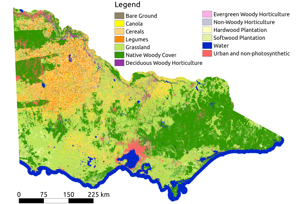
Victoria is roughly half the size of Metropolitan France. You can see the outline of the Tasman sea in the south, with the city of Melbourne and its bay along the coast in the middle. You can also see a large forested area to the east of Melbourne and up to the border of the State (in the darker shade of green), which corresponds to the Victorian Alps (yes we have Alps as well!). In the north west, a very large agricultural area (orange and yellow) and in the tip of the north-west corner: the desert!
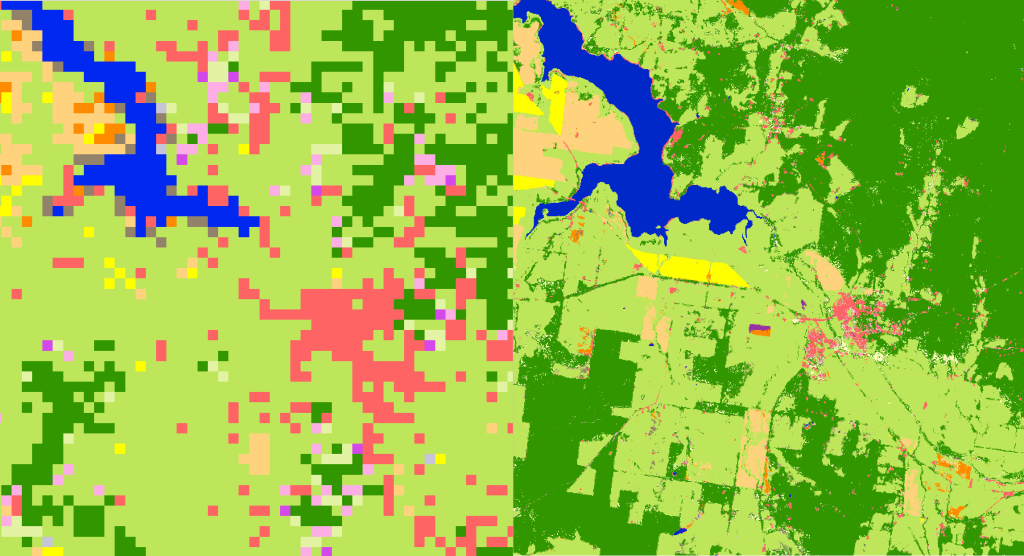
This is the first map of Victoria created at 10 m resolution – the previous one had been created from MODIS data, ie at 250 m resolution.This is what the before/after looks like.
How did we do it?
Basically, we followed the work that had been done at CESBIO with IOTA-2, but did redevelop our own scripts around OTB, and used our house-developed TempCNN algorithm, developed by Dr Charlotte Pelletier (formely at CESBIO) while at Monash University. Here are the main steps we followed:
- Download all Sentinel-2 images from July 2017 to August 2018 (winter to winter). Our job here was made much easier than it should have been, thanks to the PEPS team. We wanted good-quality LEVEL-2A data, and the PEPS servers made it possible to download 4,000+ images, across 37 tiles, directly with atmospheric corrections and cloud masks, using the on-demand MAJA processing.
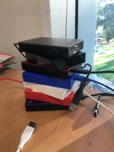
- Preprocessing. All 20 m bands were re-interpolated at 10 m (we left the 60 m ones out), stacked into 2 cubes (one for the images, one for the masks), then we interpolated the cloud-covered values using linear temporal interpolation. All of this was done using the wonderful OTB. As an aside here, our NFS had issues during the production, and so we had to resort to using 7x4TB hard drives…
Tada! You can have a play with the map yourself at http://MonashVegMap.org
Reflecting on the exercise
From start to finish, creating the map took us about 6 months, with a first iteration of the map created within 3 months and then slowly iterating through a second version. Overall, we felt that we didn’t have a good idea of the time preprocessing would take: download and preprocessing took us about 7 weeks, and this was while we were already getting L2A images. Definitely some time was lost in inputs/outputs to disks, which I believe IOTA doesn’t do as much as what we’ve done. Overall, it was quite amazing to see that this process ‘just worked’ – very well done to the team led by Jordi a few years ago and now Sen2agri. The uptake has been very positive here with numerous government bodies already using the map in their GIS, be it for fire modelling, water catchment or agricultural planning.
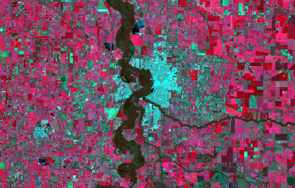
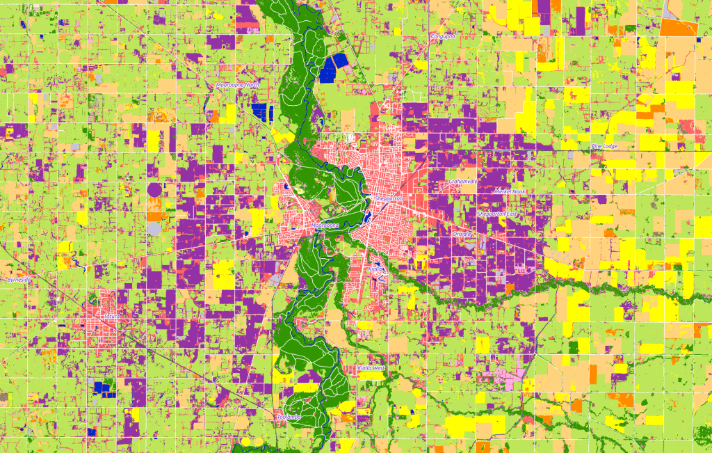
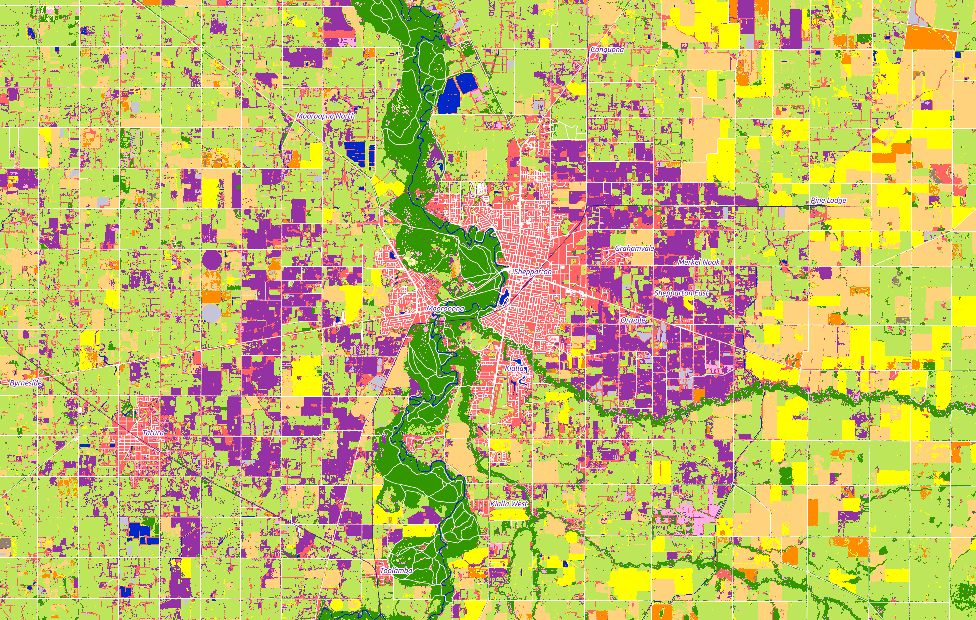
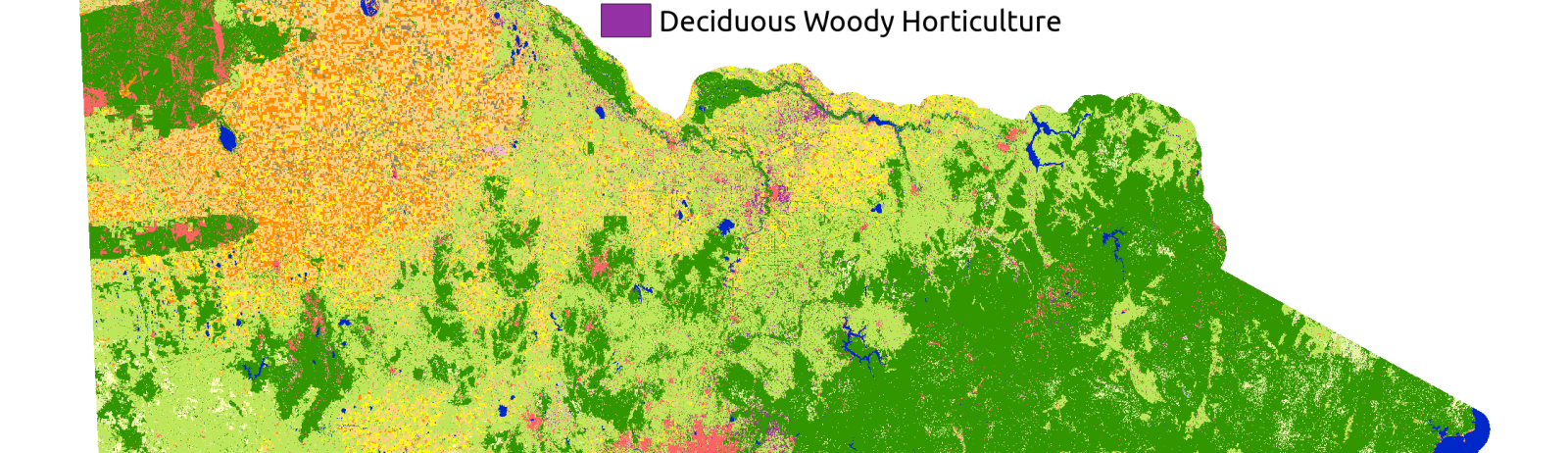
I cannot finish this post without a beautiful picture of the city of Shepparton, north of Melbourne where we grow some beautiful Shiraz (in purple) – a big recommendation if you travel to Australia and want to visit some wineries.