Sentinel-2 time series are smooth !

=> 

In a previous post, I showed a time series of pixels showing the good data quality of time series we get with Sentinel-2, processed to Level 2A by THEIA using MACCS  processor. However, I concluded that the plot I showed still had some low noise, and that a part of it was due to directional effects coming from the use of data coming from two different orbits of Sentinel-2, and therefore acquired from different viewing angles. 

Directional effect correction

I am quite sure there are some skeptic ones among the readers of this blog (I know some of them…), that could imagine the small remaining noise is due to MACCS, or Sentinel2.  So I told myself I had to prove that a large part is due to directional effects, and implemented the directional correction model we developed at CESBIO for the L3A monthly syntheses products for Sentinel-2.

This model is a constant model, that considers all surfaces have the same directional effects. This assumption is obviously false, but the approximation turns out to be quite correct when restricted to the near nadir observations angles of Sentinel-2 and LANDSAT. Our model is described as « constant model » in :

 The same approach is also used in the following reference, with a much greater data set used as input. Both of them provide very similar results.Roy, D.P., Zhang, H. K., Ju, J., Gomez-Dans, J. L., Lewis, P.E., Schaaf C.B., Sun, Q., Li, J., Huang, H., Kovalskyy, V., 2016, A general method to normalize Landsat reflectance data to nadir BRDF adjusted reflectance, Remote Sensing of Environment, 176, 255-271. For the results displayed below, we used constant values of the viewing angles per S2 Tile. This assumption is not very accurate, and the use of a viewing angle per pixel should even provide better results.

Results :

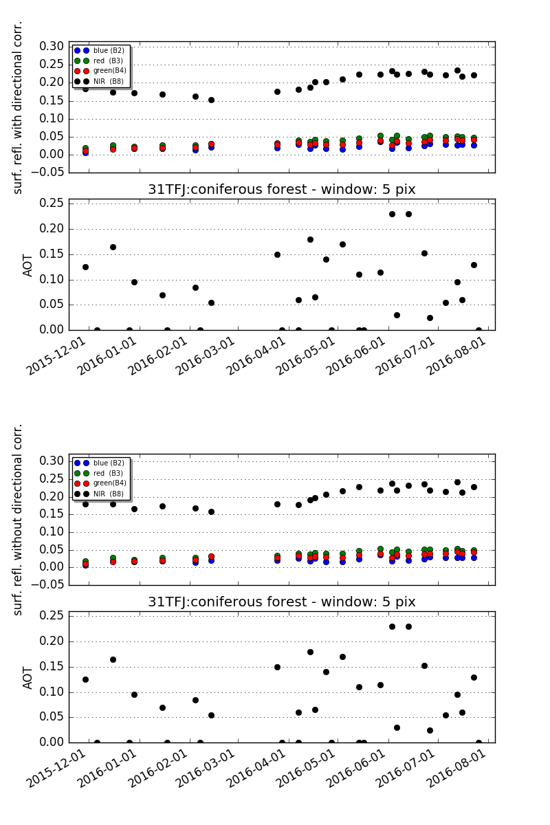
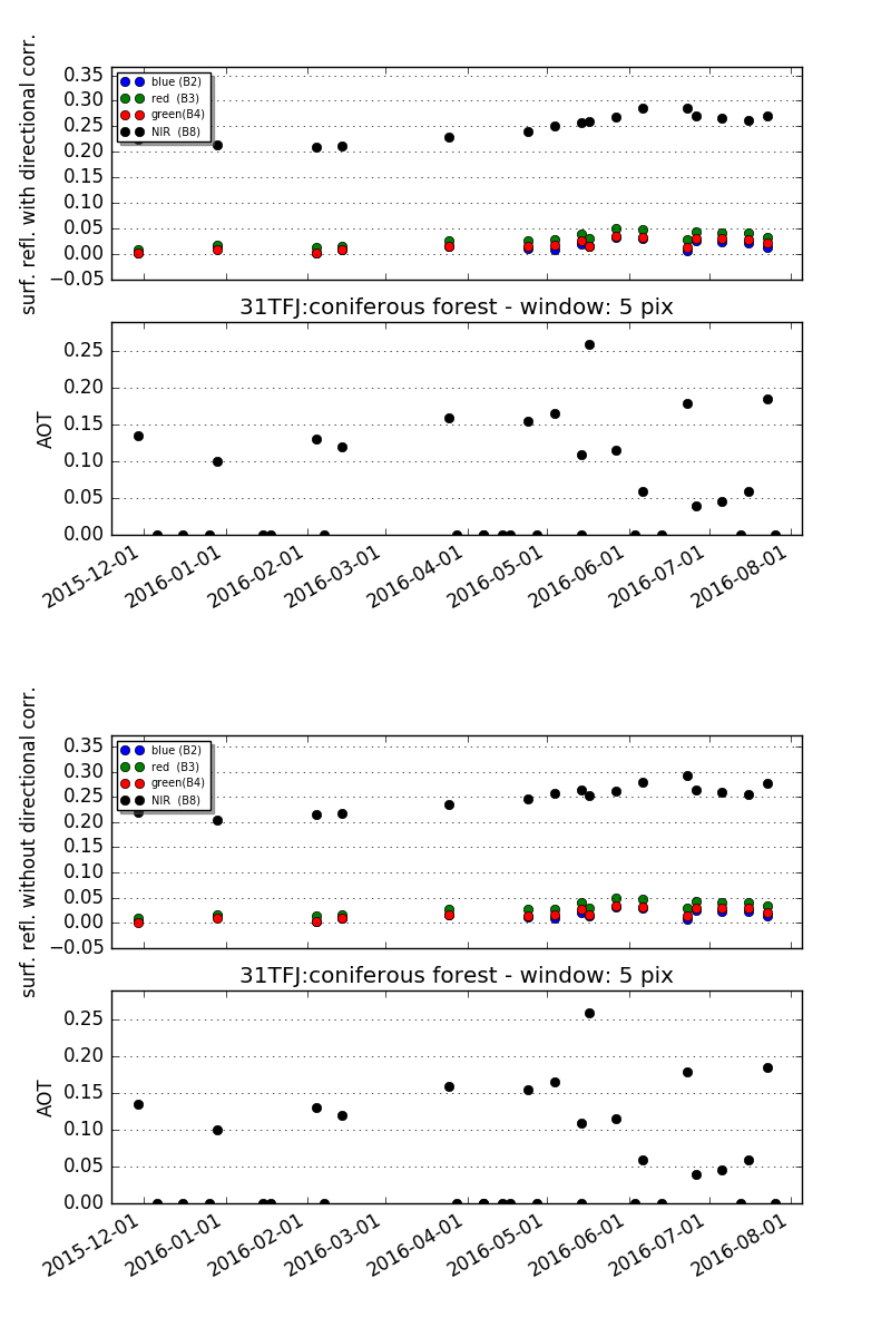
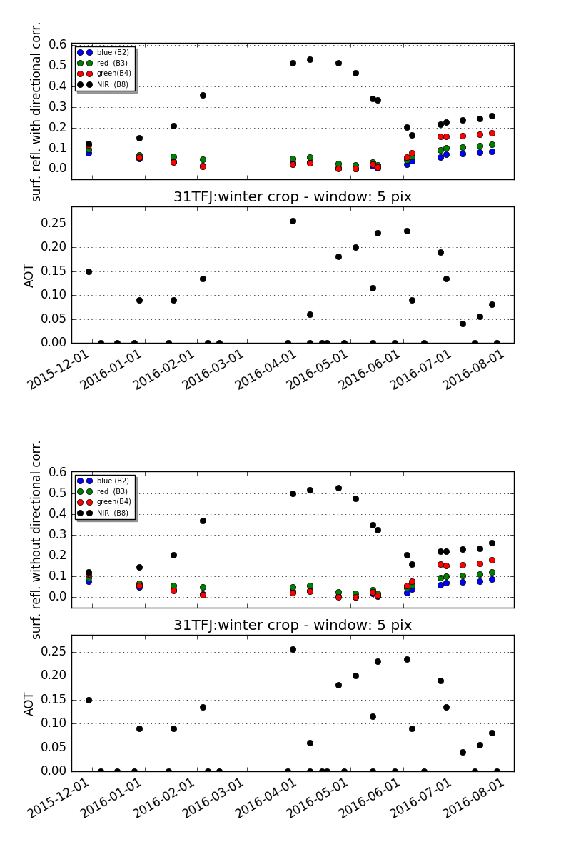
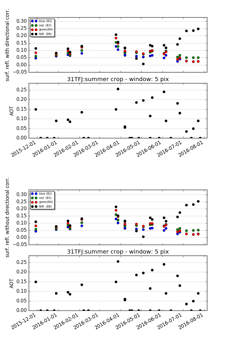
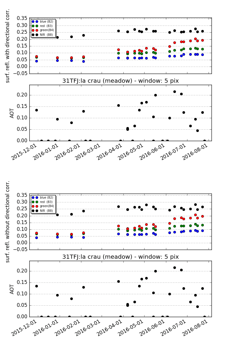
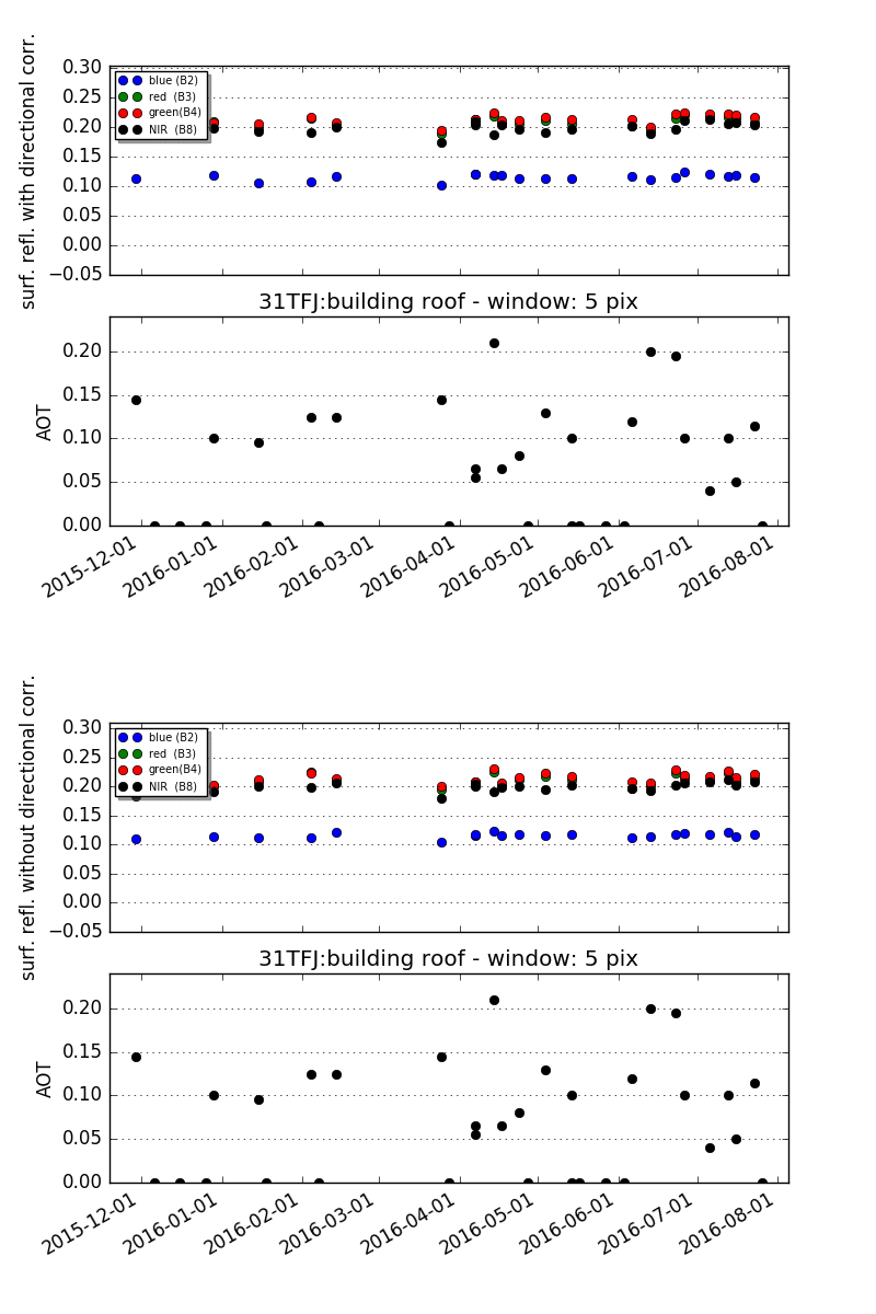
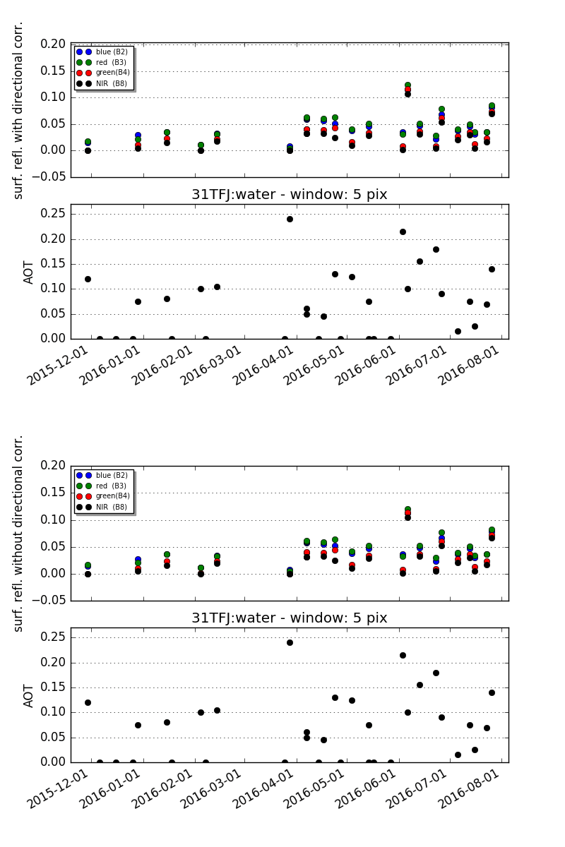
So, here are some of the results. For each figure, the top plot provides the surface reflectance as a function of time for all the 10m bands of Sentinel-2A. The bottom plot shows the AOT estimated by MACCS. If you click on the images, you will see an animation showing alternatively the results with and without directional correction. 

Comments

As it may be seen on the first 5 figures (forests, crops, la Crau), the directional correction decreases the noise, which, in the end is very low. Maybe a standard deviation of 0.01 (for a 50m x 50m aggregated pixel : given the current registration performances of Sentinel2, we can’t work at the pixel level). Of course, some anomalies may be observed. We traced some of them to an undetected thin cloud or a plane contrail shadow, but in the end, the performance is quite good. Of course, it will be enhanced with a better estimation of the angles per pixel (which is doable now, but I am a lazy one), when the L1C ortho-rectification is performed with groun
d control points, and moreover when the repetitivity of Sentinel-2 system increases with the availability of Sentinel-2B. Regarding the directional correction, the two last figures (building roof, water) don’t show enhancement related to directional correction. Our constant model is built for rough surfaces, but doesn’t work for smooth ones. This keeps up from applying it to the level 2A products, but we will distribute a tool so that you may make your own correction. And finally, the water time series seems very noisy, but this is signal and not noise : the colors of the shallow camargue lagunes change very quickly, depending on rain, wing, water level…). One very important point of the quality of the time series is the cloud and cloud shadow detection.  If you want to process large regions, such as France for instance,  you can’t spend a long time checking the quality of each cloud mask visually. And a forgotten cloud would completely ruin the quality of a time series. For this reason, our cloud masks and cloud shadow masks are very strict. and for instance, each cloud is dilated by a 400 meter buffer in order to reduce the risk of missing a thin cloud.