Bulletin GPoM-epidemiologic
The epidemic of Covid-19 and its bulletins
In this post, a brief analysis of the epidemic of Coronavirus Covid-19 that broke out in Wuhan (China) on last December 2019 is sketched. More specifically, this analysis originally focused on the period January 31st to February 27th and was then extended by Bulletins.
Bulletins
Last Bulletin:
Paper:
Supplementary Materials 1-9 MangiarottiEtAl_EpidInf2020
Archives:
Bulletin no1 (February 9), Bulletin no2 (February 26), Bulletin no3 (6 March) erratum, Bulletin_no4_(March 9), Bulletin_no5 (March 15), Bulletin no6 (March 26), Bulletin no7 (March 29), Bulletin no8 (April 2), Paper preprint (April 15), EpidInfSuppMat (April 15), Bulletin no9 (April 29), Bulletin no10 (May 6)
Context
The early development of the outbreak of Corovavirus Covid-19 (initialy called nCov) was first monitored by the Wuhan Municipal Health Commission. By the end of January, while the epidemic had started to spill over into other provinces in China, the data were then monitored at national scale and made available by the Chinese National Health Commission. Most of the data presented in the present study were gathered from this site for the present analysis.
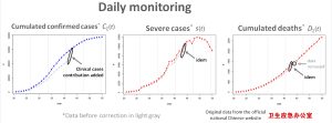
Three time series have been considered from this data set to model the propagation of the epidemic: (1) the number of cumulated confirmed cases CΣ(t), (2) the current number of severe cases s(t), and (3) the cumulated deaths DΣ(t). Their time series are shown hereafter. Note that a new methodology including the clinic cases was used after February 11. For this reason, a correction was applied to the time series on the period ranging from Day of Year 21 to 42 (around +30% for CΣ(t), +10% for s(t) and DΣ(t)).
The global modelling technique was used to obtain a model from these three variables. This technique aims to obtain sets of equations of the dynamic directly from observational time series (https://doi.org/10.1063/1.5081448, see also Actualité de l’INSU mars 2019). This technique has been applied recently to model the epidemic-epizootic coupling between human and rats for plague in Bombay (1896-1911) and for the epidemic of Ebola virus desease in West Africa (2013-2016). However, the results could be shared only after these outbreaks had stopped. Interestingly, its application to the present epidemic of Covid-19 enabled to obtain a set equations during the outbreak.
Results
The first results were obtained on February 6 and shared with other colleagues from CESBIO and ASTRE labs while the outbreak had not reached its highest peak of propagation. At this date, this preliminary analysis suggested that the epidemic was close to reach its stationnary regime and that the earlier behavior did correspond to a transient. The highest peak of propagation was attained the day after, as confirmed later. The first bulletin was diffused on February 9 (Bulletin no1) while the decrease had just started. An update of this bulletin was published online two days ago (Bulletin no2).
The simulations using the model obtained on February 6 are shown (in colour) on the following Figure where observations are also reported in black. The first time series shows that the peak of confirmed cases per day (after corrections applied) was reached on February 6 (Day of Year 37) after which a decrease started. Obviously, the maximum number of cases per day was overestimated by the model; nonetheless, the model clearly detected that the end of the transient was very close. The second time series corresponds to the number of additional severe cases per day. This reveals large oscillations that are reproduced by the model (although smaller in amplitude and speed). Finally, the third time series corresponds to the number of deaths per day. Although their maximum level is slightly underestimated in magnitude by the model, simulations appear consistent with the observations.
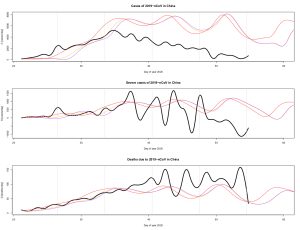
For the three variables, it is observed that a small difference in the initial conditions can lead to very different trajectories, even using fully deterministic equations. This is characteristic of chaos: a behavior at the same time deterministic and unpredictable at long term.
Another representation can be used to monitor the epidemic. The phase space (or state space) enables to represent all the states of a dynamical system. When this space is reconstructed from time series, it provides a trajectory presenting the successive states visited by the studied system. Three different projections of this phase space reconstructed from the model trajectories (colour lines) are presented on the next Figure, each starting from slightly different initial conditions. The simulations are the same as the ones presented in the last Figure, only the representation differs here. Although the time evolution was obviouly different in a temporal projection, it is clearly observed in this representation that, after a short transient, these three trajectories (in red, orange and purple) do clearly converge to the same geometrical structure. It is one typical interest of this representation: it enables a geometrical representation independent to the initial conditions. The initial conditions are different, but the dynamic is strictly the same (same deterministic equations); for this reason, the three trajectories do converge to the same geometrical structure, here, a chaotic attractor. Although these three trajectories will visit the same chaotic attractor, they will visit it in a different way, leading to an unpredictable behavior in the time space.
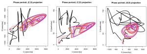
The observed trajectory is also superimposed in black which shows that the transient was modelled correctly. Although the model drawbacks previously evoked can be retrieved here (maximum number of infections per day overestimated at the maximum peak, maximum number of daily deaths slightly underestimated), it can also be noticed that the number of deaths per day did experience a succession of oscillations as suggested by the chaotic attractor (see the third projection). Differences between observed and modelled dynamics remain large. In particular,the observed signal appear much noisier than the modelled one which underlines the difficulty to handle this type of dynamical behavior. It may be noted that the model was obtained rather early, it could not take into account the most recent human action to slow down the disease, which may contribute to explain the higher maximum of infections simulated by the model.
Geographical differences
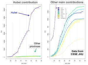
To compare the behaviors geographically, another data set made available by the Center for Systems Science and Engineering (CSSE, Johns Hopkins University) was used which provides almost online information about the spill over of the Covid-19, at global scale, and province by province for China.
Very important differences are observed from one place to another. Actually, most of the cases of Covid-19 are found in the Hubei province (65596 cumulated confirmed cases presently). The provinces the most affected after Hubei are the Gouangdong (1347), Henan (1272), Zhejiang (1205), Hunan (1017), Anhui (989) and Jiangxi (934) provinces where the number of confirmed cases is close to fifty times lower, that is, relatively much more moderate. Note that for five other provinces (the Shandong, Chongqing, Jiangsu, Sichuan and Heilongjiang), the cumulated number of confirmed cases is ranging from 400 to 800 whereas it is lower in all the other chinese provinces.
Forecastings
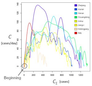
A focus of infection by the Covid-19, characterized by a quick increase of confirmed cases and deaths, has recently broken out in Italy (February 21-22). The phase space has been used to compare the early evolution in Italy to the evolution observed in the six chinese provinces previously mentioned. Two projections of this reconstructed space are provided here after for a period up to February 26 (Italy in red). The observed dynamics are very similar in amplitude and patterns. Based on the present data available, a similar behavior might have been expected in Italy in the days to come.
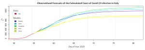
Based on this preliminary observation, the time evolution of the number of infections could be forecasted using the dynamical models obtained for the epidemic of Covid-19 in the Zhejiang, Henan, Guangdong, Anhui and Jianxi provinces. Started on February 24 these simulations suggest that the end of the epidemic may not be reached before three to four weeks, with a cumulated number of infections that would reach 800 to 1400 cases. The very last updates of confirmed cases (for February 27) however suggest that these models may probably underestimate the outbreak in Italy.
Authors
Sylvain Mangiarotti (CESBIO), Marisa Peyre (ASTRE), François Roger (ASTRE), Yàn Zhang, Mireille Huc (CESBIO), Yann Kerr (CESBIO)
Acknowledgements
This work was supported by the French programmes Les Enveloppes Fluides et l’Environnement (CNRS-INSU), Défi Infinity (CNRS) and Programme National de Télédétection Spatiale (CNRS-INSU). The extension of this work is also supported by Montpellier université d’excellence (MUSE).
References
S. Mangiarotti, M. Huc (2019) Can the original equations of a dynamical system be retrieved from observational time series? Chaos 29, 023133 (2019); https://doi.org/10.1063/1.5081448
(2015) Low dimensional chaotic models for the plague epidemic in Bombay (1896-1911). Chaos Solitons & Fractals, 81(A), 184-196 (2015); https://doi.org/10.1016/j.chaos.2015.09.014
A chaotic model for the epidemic of Ebola virus disease in West Africa (2013–2016). Chaos 26, 113112 (2016); https://doi.org/10.1063/1.4967730