A 10 m resolution land cover map of Sahel with iota2

iota2 is the large scale mapping software developed at CESBIO. iota2 takes high resolution satellite image time series (SITS), usually Sentinel (1 and 2) or Landsat, and produces maps over large areas. Maps of most usual variables of interest in remote sensing can be produced, since iota2 can compute user-defined functions at the pixel level, perform regression and classification. The main feature of iota2 is not what is computed, but the possibility of doing that on huge volumes of data (long time series, large geographical areas). Indeed, iota2 manages the image data split in tiles, the time series, the reference data for training models, the spatial stratification if needed, etc.

In the frame of the SWOT Downstream Program, a 10 m resolution land cover map of the Sahel region in Africa has been produced with iota2 using Sentinel-2 SITS covering the whole 2018 year. This amounts to 290 tiles or about 3 million km².

The map is available for download from Zenodo.

Objectives

Land cover and land use maps provide important inputs for hydrological modelling. For example, determining land-cover changes allows a better estimation on runoff ¹. Different types of vegetation and soil composition on river plains can be used to estimate river roughness in case of flood ²³. Regarding SWOT and its global coverage, large scale land cover and land use maps would foster hydrological research and downstream activities.

Can iota2 be used at a continental scale while preserving high resolution maps? What public data can be used to infer global maps? What classes are available while useful for hydrological studies? What quality level can we expect? These questions are partially addressed on this exercise.

The evaluation region includes three important basins in western Africa: Senegal, Niger and Chad basins. Such hydrographic basins extend through different countries, and in general, in situ hydrological data are out of public reach. In some other cases, basins are just insufficiently gauged. Satellite data might then provide some relevant information to better understand basin dynamics. Since such basins are affected by heavy rainy seasons and floods, a new LULC map at high resolution would help to improve runoff and flood modelling.

Data

iota2 uses supervised classification for land cover map production. For supervised classification, we need images as predictors and reference data as targets to train the classifiers.

Image data

In terms of images, we decided to use Sentinel-2 time series because of their high spatial, spectral and temporal resolution. We used the data produced by the Theia Land Data Centre over the Sahel region. These are surface reflectance image time series processed with MAJA. The area is composed of 290 MGRS tiles and we used all available dates between January and December 2018. This amounts to about 58 TB (around 200GB per tile).

Reference data

Obtaining reference data over such a large area is a difficult issue. Field surveys are out of question because of the cost of the operation. Large, well funded projects, like CGLS or WorldCover usually approach the problem via photo-interpretation, which reduces the costs, but still needs a fair amount of trained operators.

We finally decided to use existing, lower resolution maps, and settled on CGLS ⁴ as our source of reference data. Since CGLS is a 110m resolution map, using these labels for 10 m resolution images will fatally introduce some label noise. This is not very different to what is done for OSO over the classes where Corine Land Cover is used as reference data. Research shows that RF are rather robust to label noise ⁵.

Since the CGLS maps are distributed as raster data, they were vectorised so that they could be used as reference data for iota2. The vectorisation was followed by a suppression of the smallest polygons and a splitting of the larger ones so that the sampling could be efficient.

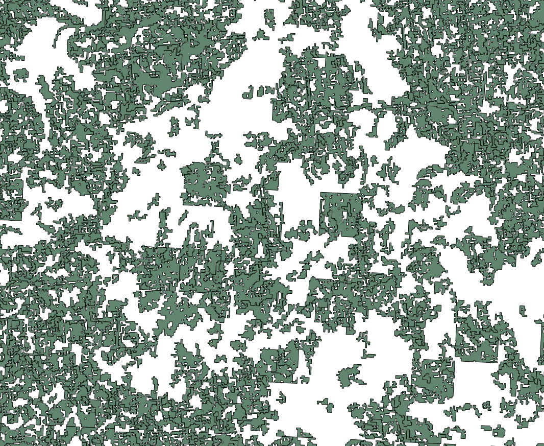CGLS raster	vectorised

Methodology

The classical iota2 workflow and its limitations

The technical details of the standard iota2 workflow for land cover mapping are described in ⁶. In a nutshell, the workflow is made of the following steps:

1. Sampling the reference data
2. Building the SITS
3. Extracting the image features for the sampled locations to generate the training data
4. Training the classifier
5. Applying the trained classifier to all the SITS

The procedure can use a geographical stratification. This approach uses a geographical partition (provided as a map, which can represent eco-climatic areas) and a different classifier is trained for each defined region. The geographical stratification serves 2 purposes. The first is to reduce the intra-class variability, which is a problem when the same thematic class has different spectro-temporal signatures on different areas. The second is reducing the amount of data, and thus the memory requirements, needed for training a classifier.

Disk space

For this exercise, it was the first time that iota2 had to process over 100 Sentinel-2 tiles for a time span of 1 year. This made appear an additional constraint: the storage capacity for all the input SITS. Indeed, for efficiency reasons, iota2 builds data stacks with all Sentinel-2 bands at 10 m resolution. This meant that we had to generate the whole map by chunks. See below for an explanation on how we proceeded.

Geographical stratification

In the case of the Sahel area, the different eco-climatic maps that we found were made of regions that were too large for the amount of disk space we had. Indeed, eco-climatic regions in the Sahel area extend in the East-West direction and a single region may intersect many MGRS tiles as shown below.

We therefore decided to generate a pseudo eco-climatic map with constraints on the region size. We used the 19 bio-climatic WorldClim variables to perform a clustering so that each region would contain a limited amount of tiles. We settled on the map below.

Each colour represents a set of climatic regions processed together. In order to avoid land cover discontinuities between the different areas, we added samples from the adjacent sub-regions for the training. In this way, adjacent classifiers have some common training samples and their decisions are similar on the boundary areas. We nearly submitted a paper to an AI journal explaining this smart strategy, but we finally decided that the Turing Award could wait.

Results

Quantitative validation

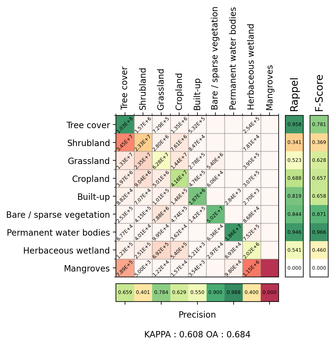
For a quantitative validation of the map, we had to rely on the CGLS map itself. As it is customary in ML, we used a hold-out set (not used for training) to compute confusion matrices. Since the reference data is a 110 m resolution raster and we produced a 10 m resolution map, we decided to produce 2 confusion matrices, one at each resolution. If we measured the quality of the map at 10 m. resolution, the discrepancies could be due to both classification errors and “super-resolution” effects. The latter correspond to the cases where the classifier predicts the correct class thanks to the 10 m resolution of Sentinel-2, but the reference data can’t contain the correct class because of its coarser resolution.

To compute the 10 m resolution matrix, we just compare the 110 m label to the 10 m pixel of the map which corresponds to the centre of the reference data pixel. To compute the 110 m resolution matrix, we first degrade the 10 m. resolution map to 110 m. by majority voting and then we compare with the reference label. Both matrices are shown below.

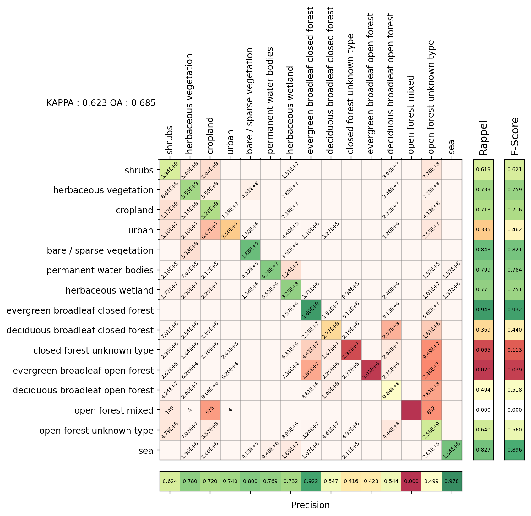confusion matrix, iota2 at 10m vs CGLS as reference

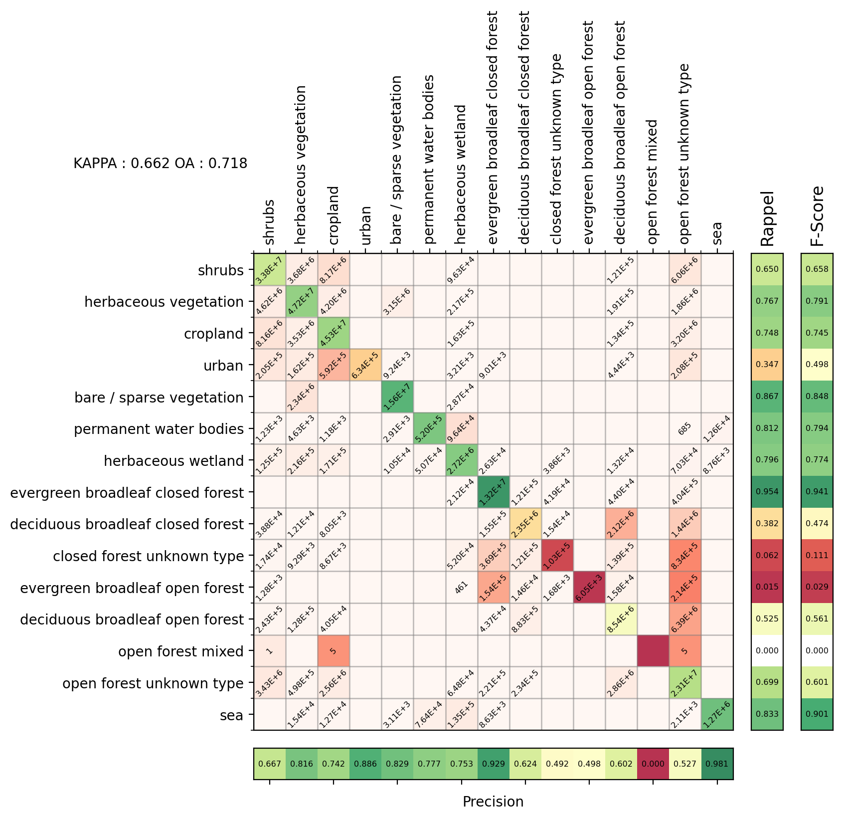confusion matrix, iota2 at 110m vs CGLS as reference

We see that the agreement between our map and CGLS increases when we compare them at the coarser resolution, as expected. However, the general trends are similar.

Qualitative analysis

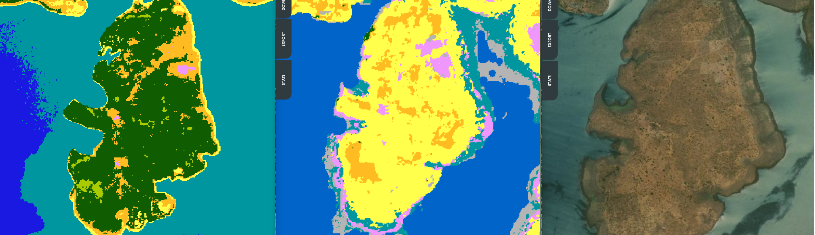
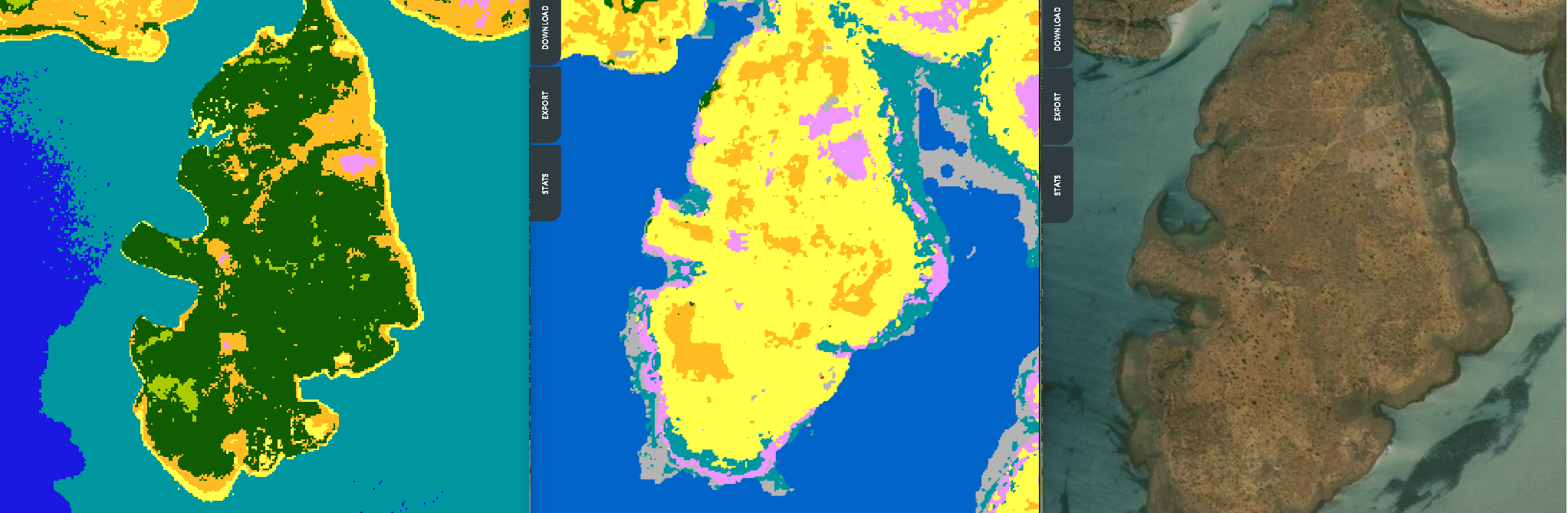
The resulting iota2 map and the original CGLS present several differences. In general, iota2 maps provide more detailed and granular results thanks to higher resolution of the inputs. Regarding the classes that would be relevant on hydrological studies, we observe that: permanent and non-permanent water areas are better delineated on iota2 maps; urban areas on iota2 maps seem less compact and present some confusion with bare ground classes, and crop areas seem also less compact and sparse than CGLS, which seems realistic in some cases. | | |:——:| | iota2 map (left), CGLS (right) |

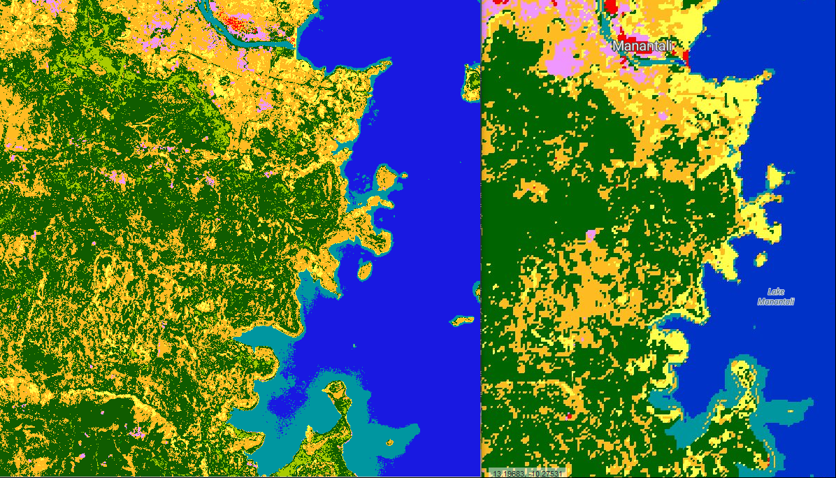iota2 map (left), CGLS (right) on Manatali Lake

Comparison with ESA WorldCover

During the final steps of the map generation, ESA WorldCover project published their global 10 m. resolution map⁷ based on Sentinel-1 and Sentinel-2 data. This map has been produced by highly qualified teams (VITO, Brockmann Consult, CS, Wageningen University, Gamma Remote Sensing and IIASA) funded by ESA. The product validation report states an overall accuracy of about 74%, which is very good for a global product. The overall approach is very similar to the one used for the CGLS product: a supervised classification using Gradient Boosting Trees of the time series using a very good set of reference data generated by trained operators.

We thought it was interesting to compare our map to WorldCover’s before dumping it into the trash bin, to see how worse our results were. We decided “validate” the ESA WorldCover with the same protocol used to validate the map produced with iota2. This allows to compare both products via the confusion matrices with respect to a 3rd one (the CGLS map). The confusion matrices obtained for the WorldCover over the region where the iota2 map was produced are shown below.

Confusion matrix, ESA product (10m) vs CGLS as reference

Confusion matrix, ESA product (110m) vs CGLS as reference

We see that the accuracy scores are slightly worse than those of iota2. Of course, this can be due to several reasons: the WorldCover map could actually be better than CGLS. Also, the comparison may not be fair, since the iota2 classifier was trained on a hold-out set of CGLS. However, these results are coherent with an independent, expert validation of our map and WorldCover’s on a small area around Lake Chad.

Qualitative comparison with ESA WorldCover

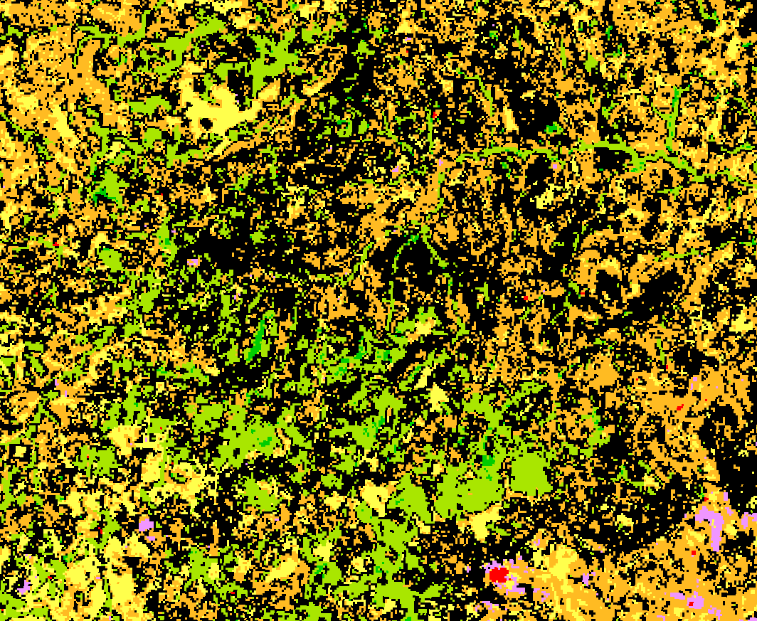
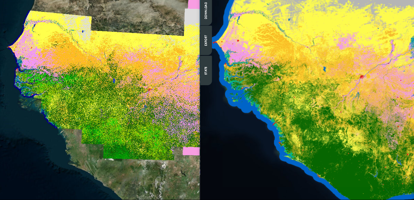
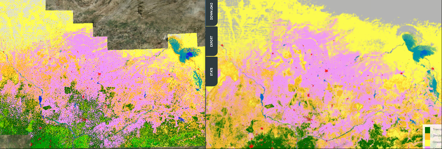
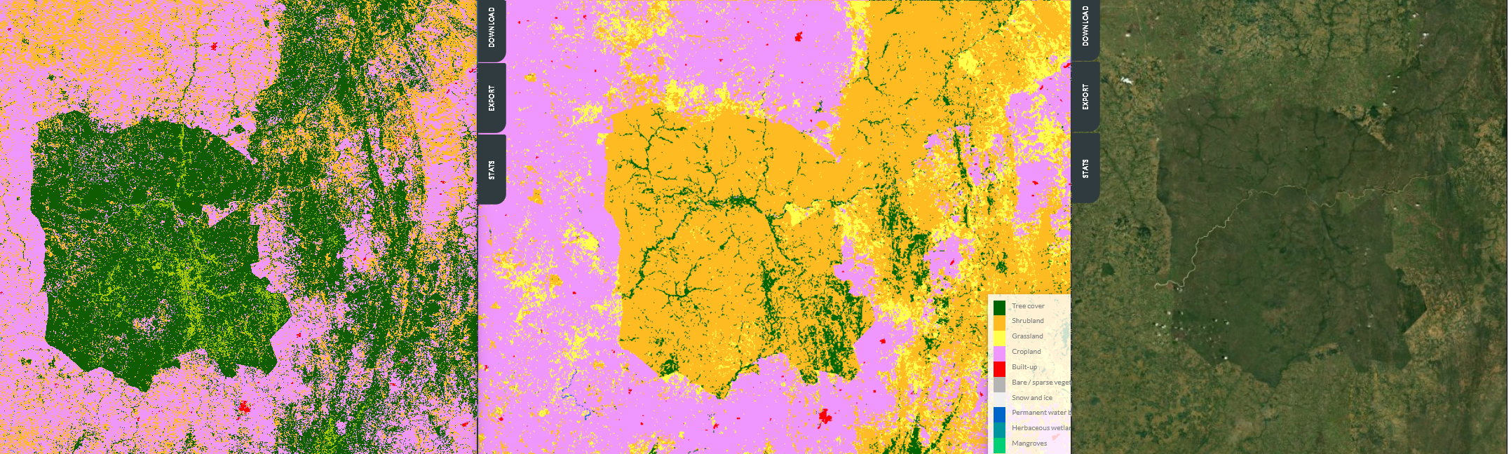
At a large scale, the geographical distribution of majority classes look similar. However, iota2 maps are less homogeneous and look more granular in transition areas. Let’s take a look at each class: vegetation and tree cover classes seem to differ, shrub (orange) and forest (dark green), probably caused by different training samples or/and class definition criteria. Water classes seem better delineated on iota2 maps, especially non-permanent water. Urban classes are clearly better defined on ESA Worldcover, being more homogeneous and having less mis-classifications as bare soil.

Comparison at large scale: iota2 map (left) vs ESA World Cover (right)

Large scale comparison at central Western Africa: iota2 map (left) vs ESA World Cover (right). Urban areas look more compact in ESA World Cover

Closer view on vegetated areas: iota2 map (left) vs ESA World Cover (right). Shrub and forest class definition seem different

Closer view on vegetated areas: iota2 map (left) vs ESA World Cover (right). Water classes delineation look better. Shrub and forest class definition seem different

Lessons learned

We have found an innovative solution for land cover mapping over very large areas without deploying costly field surveys or intensive photo-interpretation campaigns. Indeed, leveraging existing maps at lower resolution, for which reference data was used, we have produced a high spatial resolution product which seems to be on par with similar products for which reference data was specially collected.

The current study was limited by the lack of reference data for the validation step. This has 2 main consequences:

1. it is impossible to give an accurate assessment of the quality of the product;
2. we can’t determine whether the disagreements with the CGLS maps come from classification errors or from the increased spatial resolution of our product.

Unfortunately, the reference data collected for existing products are not publicly available in spite of the fact that some of them (CGLS or WorldCover, for instance) are funded with public money. This kind of data could have been used to assess the quality of our product.

From the hydrological perspective, the iota2 map seems to provide a better mapping on water areas, mainly around river-sheds and wetlands, compared to the two other global maps available (CGLS, ESA WorldCover), which would help on defining river models (river and flood plains width). Crop areas look similar between the different maps, and finally, urban and vegetated zones look better in ESA World Cover.

One could wonder why we produced this map if other products were available. First of all, the WorldCover product was not available when we started this work, but most important, one of the goals of the exercise was to assess the ability of iota2 to produce at a larger scale than the country-wide annual production for OSO. Indeed, it seems that every new land-cover initiative needs the development of a new processing chain: to the best of our knowledge, the processing chains used for CGLS, WorldCover, CCI Landcover, etc. are not open source. iota2 is free/libre software and, as such, allows study, inspection, reproducibility and adaptation to other contexts. Now we have demonstrated that it can scale beyond national mapping.

The final point worth noting is that the most burdensome part of the product generation was dealing with the huge amounts of data to be ingested by the processing pipelines. Although iota2 can jointly process Sentinel-1 and Sentinel-2 image time series, we did not use SAR data to reduce the volumes of data to use. Our past experience shows that SAR brings only small improvements for annual land-cover mapping⁸, however, these data can be useful for specific classes (i.e. urban, forest) and over tropical areas. However, the high redundancy between time series made doubling the data volume not worthy for our exercise. One way to alleviate the problem would be making available IA ready fused data, i.e. generic embeddings of multi-modal data which could be used for different downstream machine learning tasks. Imagine a 5-dimensional vector at 10 m resolution every 5 days instead of 13 reflectances every 5 days, plus 2 back-scatter coefficients every 6 days (times 2, for ascending and descending orbits), etc. This would imply a huge compression ratio, but would also simplify feature extraction and therefore less compute to train the machine learning models.

Credits

This work was carried out in the frame of the SWOT-Downstream Program. Implementation and production were done by Arthur Vincent. Algorithm design was done by Jordi Inglada. Project management and supervision were done by Santiago Peña Luque.

We are particularly grateful to CNES for the HPC infrastructure (data storage, computing resources) and CNES’ HPC technical support without whom these wonderful resources wouldn’t be operational.

The map can be cited as Vincent, Arthur, Inglada, Jordi, & Peña Luque, Santiago. (2022). Sahel Land Cover OSO 2018 [Data set]. Zenodo. https://doi.org/10.5281/zenodo.7373166

References

Sort references by citation order