[Directional effects] simple BRDF normalization
Introduction
To perform a correction of directional effect, directional models are required. A large number of directional models have been developed, such as the ones of Roujean [1] or Ross-Li [2], that try to reproduce the directional variations as a function of viewing angles and solar angles, with a rather good accuracy for most types of surfaces. Here is how they look like :
\( \rho= \rho_0 (1 + K_1. F_1(angles), + K_2. F_2 (angles))\)where \( \rho\) is the reflectance for the actual viewing and solar angles, \( \rho_0 \) is the reflectance for a given angular condition chosen to standardise the data (for instance viewing at nadir and solar angle at 45 degrees), F1 and F2 are the directional functions that depend on the angles, and \( K_1 \) and \( K_2 \) are the coefficients of the directional model, that depend on the type of surface of the observed pixel.
For wide field of view sensors, with a daily revisit, it is possible to estimate the model parameters from the satellite acquisition themselves using a period of 2 to 4 weeks, and assuming that the BRDF does not change fast [3], [4]. However, given its lower revisit and its narrower filed of view, such a method is not well adapted to Sentinel-2. The directional effects are smaller, while the time to collect 3 to 4 cloud free samples is generally greater than a month. The risk is high to confuse time variation with directional variations.
Common solution for Sentinel-2
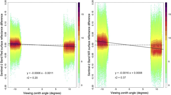
Fortunately, in the case of S2, the angle differences are low, no more than +/- 12 degrees. It is therefore possible to use constant values of the model parameters to perform the corrections. This approach has been used in [5] and [6]. In [5], we used a few acquisitions from SPOT4 (Take5) experiment obtained from two different angles to obtain constant coefficients. Roy et al did a more comprehensive study and compared Sentinel-2 observations on overlapping regions above whole countries to estimate the model parameters.

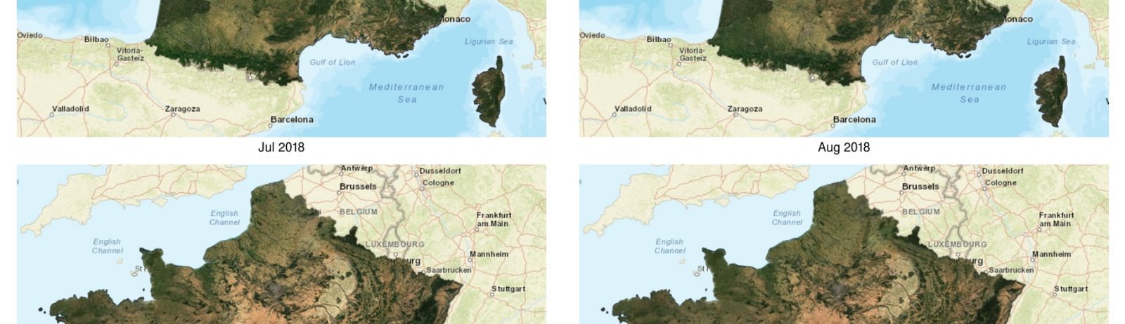
We are using the Roy et al model to normalize directional effects in our surface reflectance syntheses obtain with WASP software. The swath edges are almost invisible in the syntheses obtained in summer, which shows a good success of the Roy model.
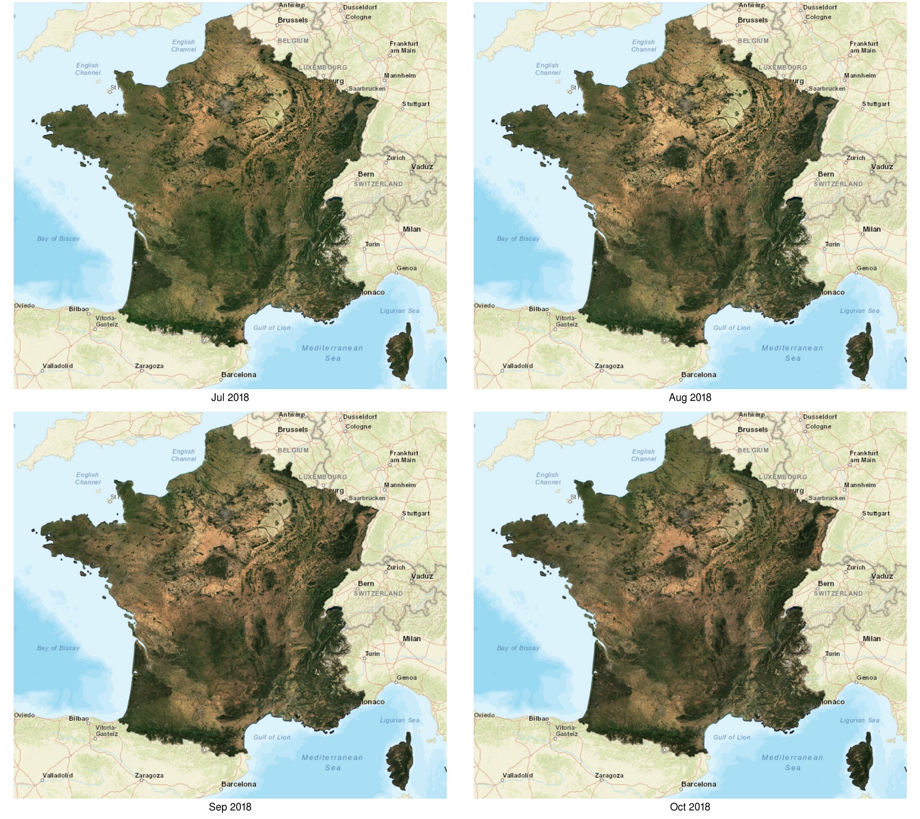
However, the Roy model does not perform as well in winter, when the sun elevation is much lower, and the edges of the swaths become visible, as shown in next figure, in which it is possible to see the limits of the swaths.
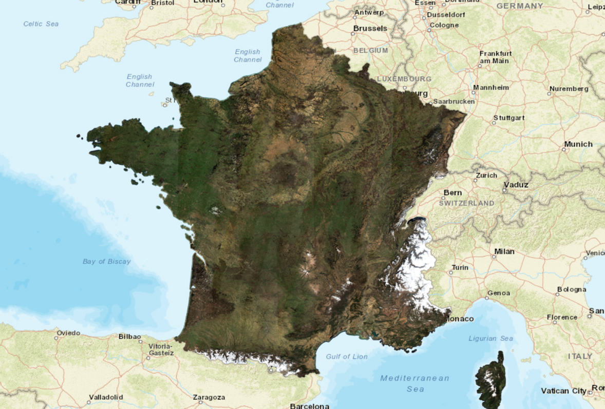
It is not fully a surprise that a model with only three parameters is not fully able to account for the complexity of directional effects. However, reading again the paper from Roy et al, I noticed that it had been built on data from South Africa, for which, even in winter, the sun is always quite high on the horizon. It means a better fit of the data based on a better sample of reflectances is possible. However, it will still be a very (too) simple model.
Verification with DART model
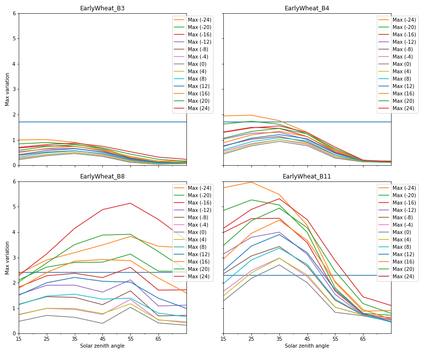
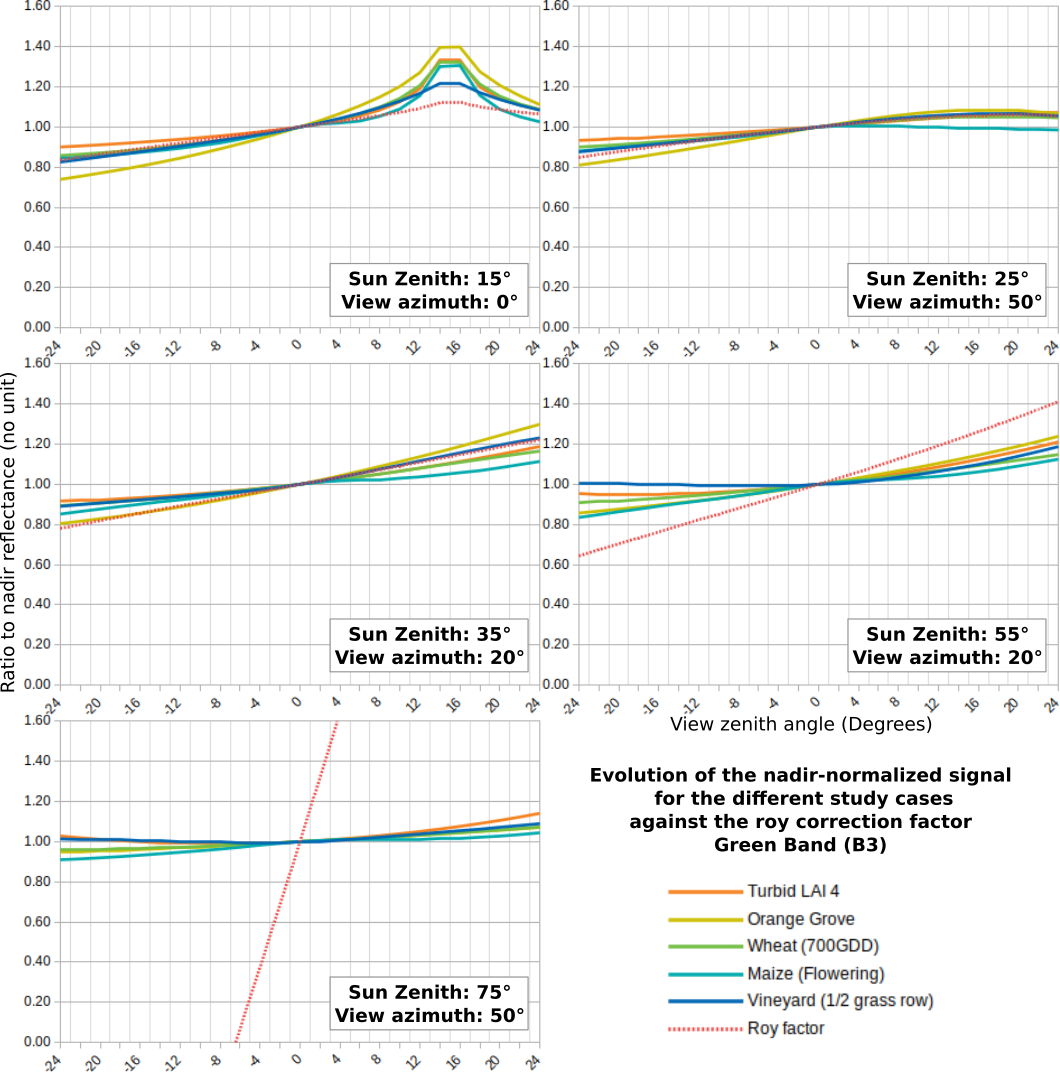
Using the simulations performed with the DART 3D radiative transfer model, detailed on this post, we compared the bidirectional variations, normalized at Nadir, of different types of vegetation covers for 4 spectral bands : green, red, NIR and SWIR (1.6 µm). The figures below show that while the Roy et al model agrees with DART simulations for solar zenith angles between 15 and 45 degrees, they start to disagree at 55 degrees, and the Roy et al model is completely wrong, as suggested by what we observed on the L3A syntheses in winter with the Roy correction.
 Green band Green band | 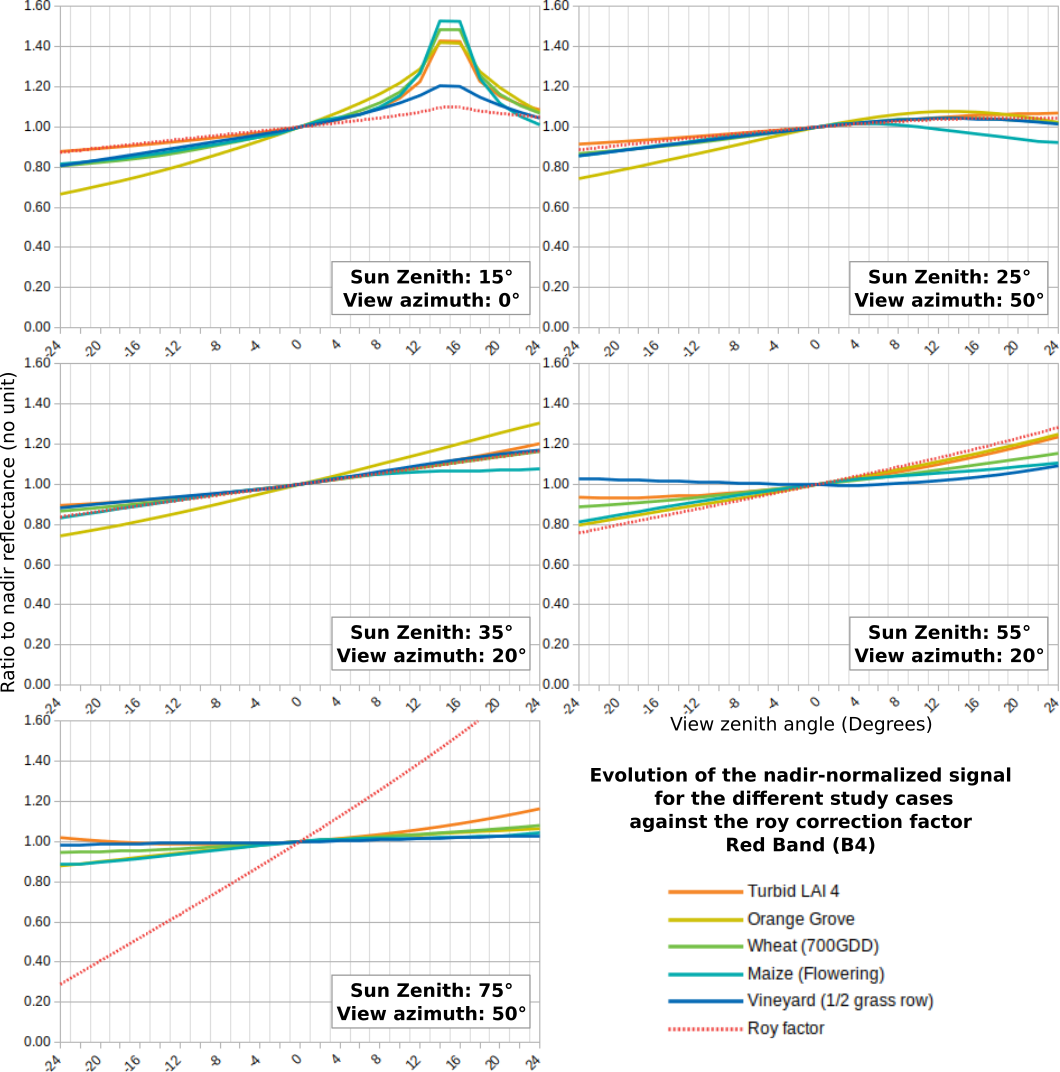 Red band Red band |
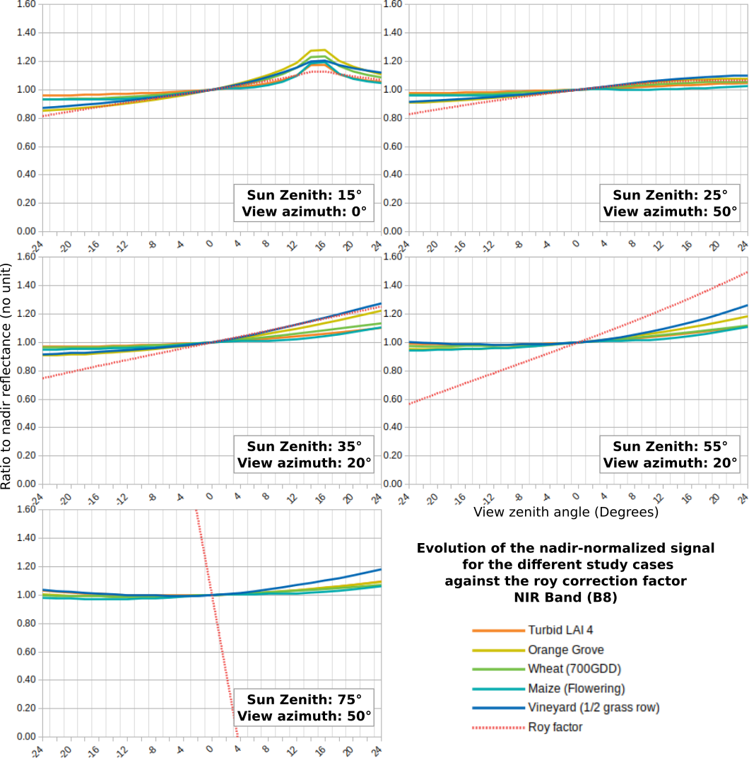 NIR band NIR band |
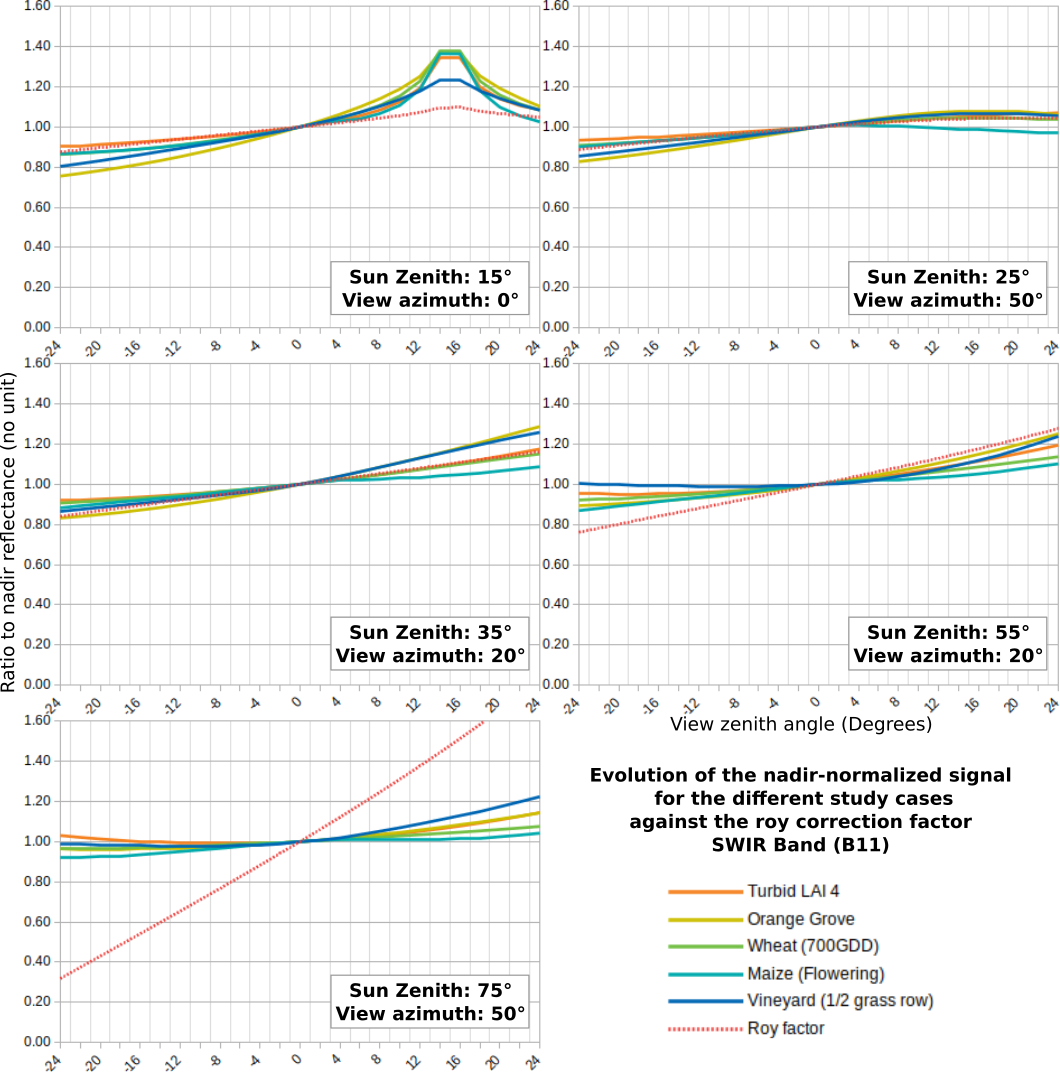 SWIR Band |
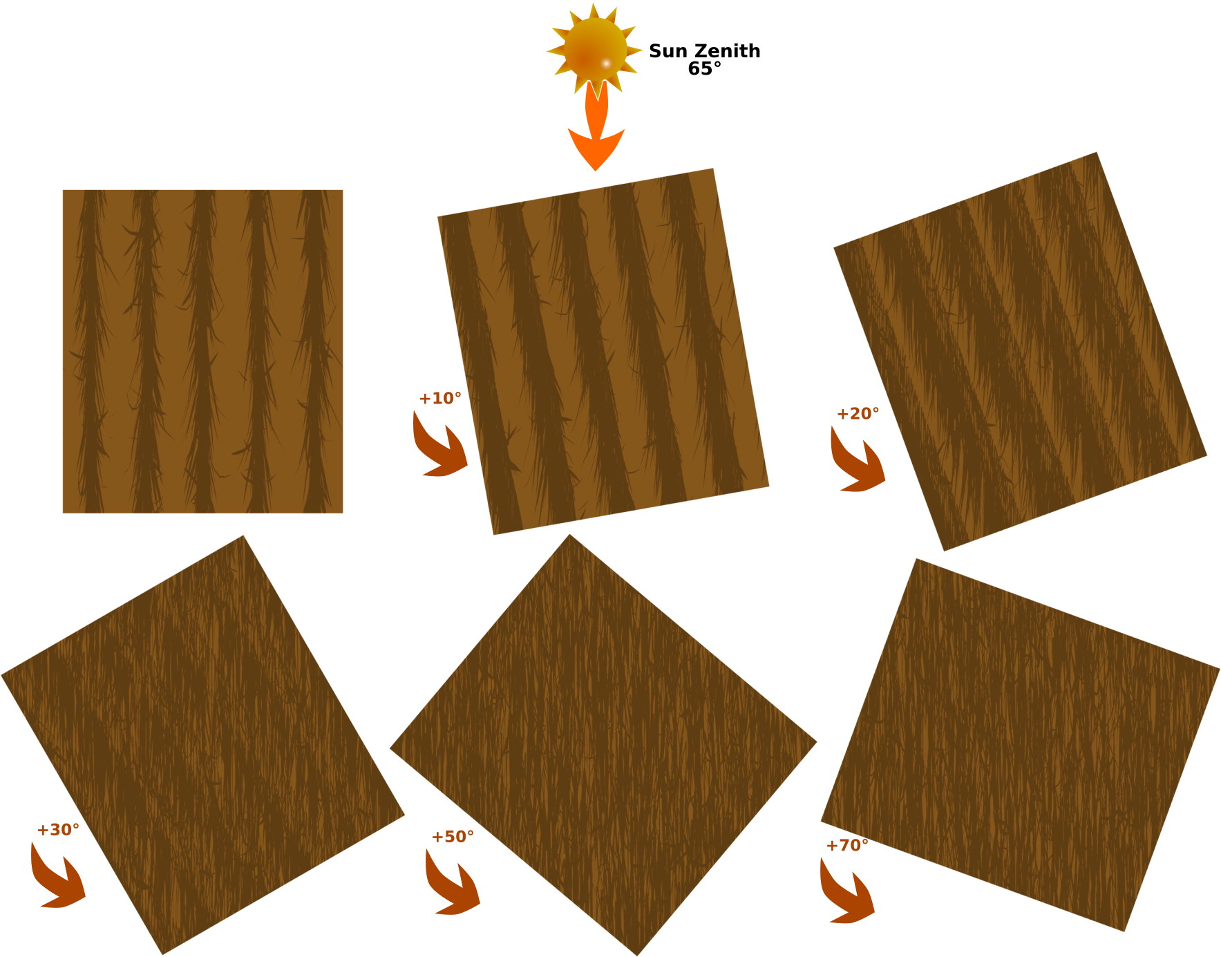
Comparison for diverse geometrical configurations of BRDF variation with regard to nadir, for DART simulations of 4 different vegetation covers, and also for a turbid vegetation, i.e a layer of uniform smashed vegetation on top of a uniform ground. The absciss is the view zenith angle, with positive angles towards backscatering (or towards the East for a morning observation satellite, and negative values towards forward scattering. The maximum viewing angle, 24° corresponds to twice the field of view of Sentinel-2.
So as a conclusion, for thef ield of view of Sentinel-2 (12°), and for sun zenith angles greater than 50°, the Roy et al model can correct fairly well directional effects for the field of view of Sentinel-2. We can also notice that the different types of vegetation already have differences of +/- 5% at the edge of the swath, which might be insufficient for some applications. The simulations also show that the scattering increases almost linearly with view angles. Finally, it is also worth noticing that the turbid simulations with a LAI of 4 is not far from an average of all the vegetations covers. As a result, it should be possible to replace the Roy model by a LUT obtained from a turbid simulation.
As said above, a new version of Roy model could be obtained by fitting it over data from higher latitudes, in order to better cover the range of sun zenith angles. But it is a huge amount of data to process …