Using NDVI with atmospherically corrected data

NDVI

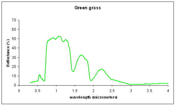
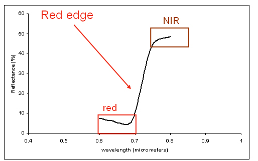
NDVI is by far the most commonly used vegetation index. NDVI was developed in the early seventies (Rouse 1973, Tucker 1979), and widely used with remote sensing in the nineties until now. It is computed from the surface reflectance in the red and near infra-red channels on each side of the red-edge.

\( NDVI=\frac{\rho(NIR)-\rho(RED)}{\rho(NIR)+\rho(RED)} \)

 where \(\rho(NIR)\) and \( \rho(RED)\) are reflectances in the NIR and RED. Although several users still use top-of atmosphere reflectances (TOA), surface reflectances should be used to reduce sensitivity to variations of aerosol atmospheric content.

I think NDVI is mainly used for the following reasons (but feel free to comment and add your reasons) :

• it has the large advantage of qualifying the vegetation status with only one dimension, instead of N dimensions if we consider the reflectances of each channel. Of course, by replacing N dimensions by only one, a lot of information is lost.
• it  enables to reduce the temporal noise due to directional effects. But with the Landsat, Sentinel-2 or Venµs satellites, which observe under constant viewing angles, the directional effects have been considerably reduced.

I therefore tend to tell students that if NDVI is convenient, it is not the only way to monitor vegetation.

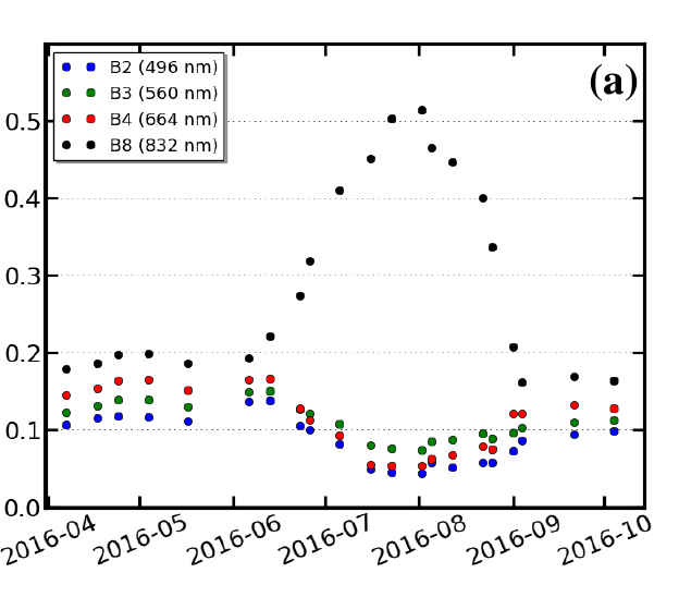
NDVI is quite sensitive to atmospheric effects, and time series of NDVI before atmospheric correction can be quite noisy if variations of aerosol atmospheric content are observed. At the time it was developed, it was not very frequent to access to data corrected for atmospheric effects. The situation has changed now, and we see much more users work with NDVI after atmospheric correction. But it also turns out NDVI has some drawbacks when used after atmospheric correction, with surface reflectances instead of TOA reflectance. The issue is that red band surface reflectances are much lower than the TOA reflectances.

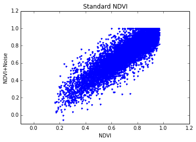
As shown in the following Jupyter Notebook (my first one !), NDVI turns out to be very sensitive to noise when surface reflectances in the red are low. Because of the noise, the reflectances can be close or equal to zero, if not negative. In that case, the NDVI gets very close to 1 whatever the NIR reflectance. And I receive quite often complaints about NDVI outliers due to very low reflectances. The usual consequence is that these users question the quality of the atmospheric correction, and even the necessity to perform atmospheric correction. Of course, atmospheric correction can be criticised, it is difficult and will never be perfect, there will always be some residual noise due to aerosol estimation errors, incomplete cloud masking, errors in adjacency effect estimates… That’s why  I think we should question the use of NDVI in its standard definition.

ACORVI

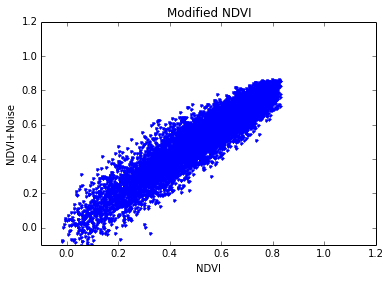
Anyway,  there is a quite simple solution to solve the issue of red surface reflectances close to zero : just add a constant to the red band surface reflectance. This constant must be greater than the standard deviation of atmospheric correction noise. As this one is usually close to 0.01, the constant could be 0.05.

\( NDVI=\frac{\rho_s(NIR)-(\rho_s(RED)+0.05)}{\rho_s(NIR)+(\rho_s(RED)+0.05)} \)

With such a definition of NDVI, we can see that the new version of the plot we had shown above looks much better below.

It is very probable that such a modified NDVI was already proposed in the litterature but I did not find it among the most famous ones (Bannary et al 1996), including the Atmospherically Resistant Vegetation Index (Kaufman et al, 1992). So maybe should I call this one the Atmospheric COrrection Resistant Vegetation Index (ACORVI)Now that I have defined my own vegetation index, I could retire happily ! I hope none of my neighbours in conferences remember that I used to say that defining a vegetation was really something of the past.

A colleague asked me what was the use of subtracting atmospheric effects if it was to add a constant afterwards. Well, atmospheric effects are variable with time, while the constant is… constant.

Conclusions

Let’s summarise:

• There is much more information in reflectances than in NDVI
• But if you still find NDVI convenient, and if you are using atmospherically corrected reflectances, you will have better results with the ACORVI index.

ESA and Nima Pahlevan from NASA do approve ACORVI 😉

References

Rouse J.W., Haas R.H., Schell J.A., Deering D.W., 1973. Monitoring vegetation systems in the great plains with ERTS. Third ERTS Symposium, NASA SP-351. 1:309-317

Tucker C.J., 1979. Red and photographic infrared linear combinations for monitoring vegetation. Remote Sens Environ 8:127-150

Kaufman Y. J., Tanre D., 1992. Atmospherically Resistant Vegetation Index (ARVI) for EOS-MODIS, I.E.E.E. T geosci remote 30(2):261-270

Bannari, A., Morin, D., Bonn, F., & Huete, A. R. (1995). A review of vegetation indices. Remote sensing reviews, 13(1-2), 95-120.

See also this impressive database of remote sensing indexes : https://www.indexdatabase.de/

PS

I found the nice graphs on top of this post from this site, sponsored by Eumetsat :http://www.eumetrain.org/data/3/36/navmenu.php?page=1.0.0

Nima Pahlevan did not authorize me for the above photograph, I hope he doesn’t mind.