Machine learning benchmarking for land cover map production

The iota2 processing chain is highly configurable in terms of how the images are pre-processed, how the reference data is prepared, how the classifiers are paremeterised, etc. We also continuously add new approaches. During this development work, we need to assess whether a change to the workflow performs better than the previous approaches. In order to do this, we use standard metrics for classification derived from the confusion matrix (Overall Accuracy, κ coefficient, F-Score). The confusion matrix is of course computed using samples which are not used for the training, but we go a little further than that by splitting the train and test sets at the polygon level. Indeed, our reference data is made of polygons which correspond to agricultural plots, forests, urban settlements, etc. Since images have a strong local correlation, pixels belonging to the same polygon have a high likelihood of being very similar. Therefore, allowing a polygon to provide pixels for both the training and test sets yields optimistic performance estimations. Most of our tests are performed over very large areas (at least 25% of metropolitan France, often more than that), which means that, using reference data from Corine Land Cover, we have many more samples than we can deal with. Even in this situation, we perform several runs of training and testing by drawing different polygons for each run, which allows us to estimate confidence intervals for all our metrics and therefore assess the significance of the differences in performance between different parameter settings. All this is good and well, but this is not enough for assessing the quality of the results of a particular algorithm. 

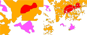
The data we feed to the classifier are images and they are pre-processed so that application agnostic machine learning approaches can deal with that. In iota2, we perform eco-climatic stratification, which can introduce artifacts around strata boundaries. We also perform temporal gapfilling followed by a temporal resampling of all data so that all the pixels have the same number of features regardless of the number of available clear acquisitions. After that, sometimes we compute contextual features which take into account the neighbourhood of the pixels, in Convolutional Neural Networks, a patch size is defined, etc. All these pre-processing steps have an influence on the final result, but most of the time, their effect can’t be observed on the global statistics computed from the confusion matrix. For instance, contextual features may produce a smeared out image, but since most of the validation pixels are inside polygons and not on their edges, the affected pixels will not be used for the validation. In our case, the reference data polygons are eroded in order to compensate for possible misregistrations between the reference data and the images. Therefore, we have no pixels on the boundaries of the objects. In our paper describing the iota2 methodology, we presented some analysis of the spatial artifacts caused by image tiling and stratification, but we lack a metric for that. The same happens when using contextual features or CNNs. The global point-wise metrics increase when the size of the neighbourhoods increase, but the maps produced are not acceptable from the user point of view. The 2 images below (produced by D. Derksen, a CESBIO PhD candidate) illustrate this kind of issues. The image on the right has higher values for the classical point wise metrics (OA, κ, etc), but the lack of spatial accuracy is unacceptable for most users.

 Even if we had an exhaustive reference data set (labels for all the pixels), the number of pixels affected by the over-smoothing are a small percentage of the whole image and they would just weight a little in the global metrics. We are working on the development of quantitative tools to measure this effects, but we don’t have a satisfactory solution yet. 

All what has been said above does not consider the quality of the reference data. At CESBIO, we have learned many things over the years about the different kinds of impacts of the quality of reference data, both in the classifier training and the map validation step. We have people here who collect data on the field every year on hundreds of agricultural plots. We have also a bit of experience using off-the-shelf reference data. The quality of the results is much better when we use the data collected by our colleagues and we have a rather good understanding on what happens during training and validation. Ch. Pelletier recently defended her PhD and most of her work dealt with this issue. For instance, she analysed the impact of mislabelled reference data on the classifier training and showed that Random Forests are much more robust than SVM. She also developed techniques for detecting errors in the reference.We also use simple ways to clean the reference data. For instance, when using Corine Land Cover polygons which have a minimum mapping unit (MMU) of 25 hectares, we use information coming from other data bases, as described from slide 34 in this presentation. An illustration of the results is shown below.

The reasons for having label noise in the reference data can be many, but the 2 main we face are: the MMU and the changes occurred since the collection of the reference data. For our 2016 map, we used Corine Land Cover 2012, and therefore, we may assume that more than 5% of the samples are wrong becau
se of the changes. Therefore, when validating with this data, if for some classes we have accuracies higher than 95%, we must be doing something wrong. If we add the MMU issue to that, for the classes for which we don’t perform the cleansing procedure illustrated above, accuracies higher than 90% should trigger an alarm. Our ML friends like to play with data sets to improve their algorithms. Making available domain specific data is a very good idea, since ML folks have something to compete (this is why the work for free for Kaggle!) and they provide us with state of the art approaches for us to choose from. This is the idea of D. Ienco and R. Gaetano with the TiSeLaC contest: they used iota2 to produce gapfilled Landsat image time series and reference data as the ones we use at CESBIO to produce our maps (a mix of Corine Land Cover and the French Land Parcel Information System, RPG) and provided something for the ML community to easily use: CSV files with labelled pixels for training and validation. The test site is the Reunion Island, which is more difficult to deal with than metropolitan France mainly due to the cloud cover. Even with the impressive (ahem …) temporal gapfilling from CESBIO that they used, the task is difficult. Add to that the quality of the reference data set which is based on CLC 2012 for a 2014 image time series, and the result is a daunting task. Even with all these difficulties, several teams achieved FScores higher than 94% and 2 of them were above 99%. It seems that Deep Learning can generalise better than other approaches, and I guess that the winners use these kind of techniques, so I will assume that these algorithms achieve perfect learning and generalisation. In this case, the map they produce, is perfect. The issue is that the data used for validation is not perfect, which means that an algorithm which achieves nearly 100% accuracy, not only has the same amount of error than the validation data, but also that the errors are exactly on the same samples! I don’t have the full details on how the data was generated and, from the contest web site, I can’t know how the different algorithms work ², but I can speculate on how an algorithm can achieve 99% accuracy in this case. One reason is over-fitting³, of course. If the validation and training sets are too similar, the validation does not measure generalisation capabilities, but it rather gives the same results as the training set. Several years ago, when we were still working on small areas, we had this kind of behaviour due to a correlation between the spatial distribution of the samples and local cloud patterns: although training and test pixels came from different polygons, for some classes, they were close to each other and were cloudy on the same dates and the classifier was learning the gapfilling artifacts rather than the class behaviour. We made this mistake because we were not looking at the maps, but only optimising the accuracy metrics. Once we looked at the classified images, we understood the issue. 

In this era of kaggleification of data analysis, we must be careful and make sure that the metrics we optimise are not too simplistic. It is not an easy task, and for some of the problems we address, we don’t have the perfect reference data. In other situations, we don’t even have the metrics to measure the quality.The solutions we use to solve mapping problems need an additional validation beyond the standard machine learning metrics.