Adjacency effects, or how pixels from the entire region can skew your measurements

=>

Neighborhood issues also exist in Earth observation. And in a sense, they are even much more serious than on a social level, since neighbors located more than 30 km away can cause interference! Fortunately, we have the means to correct these problems without resorting to law enforcement—just using algorithms.

This entire article is based on Kevin Walcarius’s insightful research on what we call atmosphere-related adjacency effects. Kevin has just completed a postdoctoral fellowship for CNES at the CESBIO laboratory, under my supervision. This work was supported by the HYGEOS company, which was also funded by CNES through its R&T program. The scientific article resulting from this research has just been published in Remote Sensing Environment.

This blog already includes a post on adjacency effects, written a little over 10 years ago, but our understanding of the phenomenon has changed somewhat thanks to Kevin’s work. After outlining the problem, this blog post presents the main conclusions of the article.

Adjacency effects

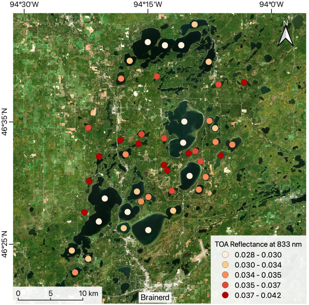
The illustration below, taken from an article by Wu et al., shows the magnitude of these adjacency effects. In the near-infrared (NIR), water strongly absorbs light; therefore, the surface reflectance of lakes should be very close to zero and fairly uniform across the entire image. The colored dots represent the PIR reflectance values at the top of the atmosphere, at the center of numerous lakes. We observe that the smaller the lake, the higher its apparent reflectance. Adjacency effects are the cause of this phenomenon, and the image clearly shows that these effects are all the more pronounced the closer and brighter the surrounding area is (in the near-infrared, vegetation is very bright, while water is dark).

Le graphique ci-dessous explique bien le phénomène :

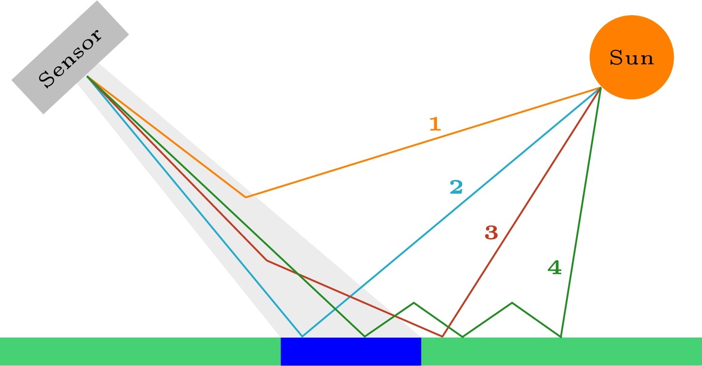
Suppose we observe the blue pixel in this graph using an optical satellite. The photons of interest to us are those that follow path type 2, with a direct interaction at the pixel’s surface and no interaction with the atmosphere. Unfortunately, some of the photons detected by the satellite seemingly coming from our blue pixel, actually come directly from the atmosphere, without interacting with the ground (path 1). They can also result from an interaction with the atmosphere, after reflection on the surrounding area (path 3), or from multiple interactions between the atmosphere and the ground (path 4). Because of paths 3 and 4, our satellite’s measurement for the blue pixel is therefore sensitive to its surroundings. This is known as the “adjacency effect.”

Atmospheric effects can be modeled using the formula below. The colors used in the formula correspond to those in the graph above: blue represents Type 2 paths, orange represents Type 1 paths, purple represents Type 2 paths, and green represents multiple Type 4 paths:

$\rho_{TOA}$ is the reflectance observed at the top of the atmosphere, $\rho_{atm}$ is the reflectance due to scattering in the atmosphere, $\rho_s$ is the surface reflectance, which we are seeking, and $\rho_{env}$ is the environnement (or adjacency) reflectance. Finally, T represents the transmittance—attenuation factors associated with the path through the atmosphere—on the downward path, indicated by downward arrows $T^\downarrow$, and on the upward path, indicated by upward arrows. The suffix “dir” corresponds to the transmittance along the direct path (type 2), and “dif” to the transmittance along the diffuse path (type 3). Finally, « a » is the albedo of the atmosphere, and the denominator corresponds to path type 4.

Although this is an approximation, the environmental reflectance is commonly modeled as a convolution of the surface reflectance $\rho_s$ with a point spread function $P_{env}$.

To compute the point spread function, the observed scene must be modeled in 3D using Monte Carlo radiative transfer codes. A simulation involves emitting photons and tracking their paths and interactions with the surface and the atmosphere. The more photons that are emitted, the more accurate the result. When the first environmental effect models were developed in the 1980s or 1990s (Tanré et al., Vermote et al.), launching 10,000 photons already took several minutes. The accuracy of the calculations was therefore low, and the models found that the range of these environmental effects was on the order of one or two kilometers. That’s why, until now, in our MAJA atmospheric correction software, we had been using a Gaussian distribution with a standard deviation of 330 m, and thus a maximum distance of 1 km.A bright pixel therefore seemed to have virtually no effect beyond 1 km. However, observations (Bulgarelli et al.) have shown that coastlines can interfere with maritime observations of reflectances at distances of about 30 kilometers.

Lorsque les premiers modèles d’effets d’environnement ont été mis au point dans les années 80 ou 90 (Tanré et al, Vermote et al), lancer 10 000 photons prenait déjà des minutes. La précision des calculs était donc faible, et les modèles ont trouvé que la portée de ces effets d’environnement étaient de l’ordre d’un ou deux kilomètres. Jusqu’ici, dans le logiciel de correction atmosphérique MAJA, nous utilisions donc une gaussienne avec un écart-type de 330m, et donc une distance maximale de 1 km.

This is what prompted us to redo the calculations using HYGEOS’s SMART-G code, which, thanks to powerful GPUs, can launch one billion photons per second. The results we obtained are quite different from those obtained 30 years ago. Our results confirm those observed by Bulgarelli et al. Other colleagues, Wu et al. (2024), also developed a model of adjacency effects based on a Monte Carlo code; however, to greatly simplify their calculations, they did not take into account path type 4, which is a correct assumption over dark water, but is quite wrong over bright land.

Point spread function computation, and sensitivity analysis

To determine the point spread function (PSF), the easiest approach would be to use a uniform neighborhood and observe how a single white pixel influences its surroundings. However, this method is not efficient, because if we emit billions of photons from the sun, most of them will strike the dark region, be absorbed, and therefore will not contribute to the calculation of the PSF. We therefore decided to use larger bright targets (Gaussian functions of various sizes) and let the processing handle the separation of the source effect and the impulse response. This operation is generally a difficult problem to solve because it is highly sensitive to noise, and we solved it by assuming that the PSF follows an analytical model with only two parameters. It is the King model, quite commonly used in optics, that provided the best results.

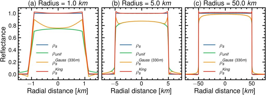
The results below compare three methods of adjacency effect correction for artificial targets consisting of disks of different radii: a method that assumes a uniform landscape and does not account for adjacency effects; the method currently used in MAJA, which uses a Gaussian PSF with a spread of 1 km (standard deviation of 330 m); and King’s PSF, as determined in this study.

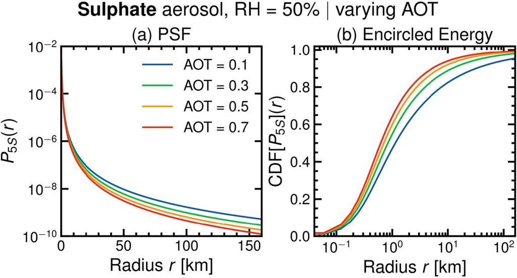
The following figure shows the King PSF obtained for an atmosphere containing fine sulfate aerosols, for four values of optical depth (AOT). It is interesting to note that the fewer the aerosols, the longer the range of the impulse response because when the AOT is high, more frequent interactions with the aerosols prevent light from scattering too far. Nearly 5% of the adjacency effects can extend beyond a radius of 100 km for a small AOT equal to 0.1.

Validation of our adjacency effect correction

The results shown so far were obtained using artificial landscapes (disks), which are not realistic; the derived orders of magnitude are therefore not realistic either. In the following section, we validated our results in two ways:

• using natural landscapes, but still based on simulations
• using real images from Sentinel-2, corrected for environmental effects, and compared to in-situ measurements of marine reflectance

Validation with simulations using a real landscape

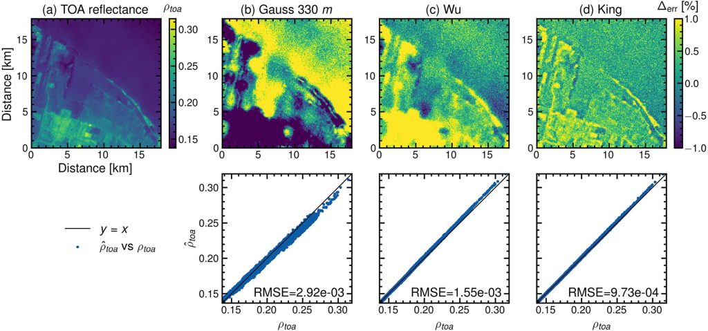
For the result below, Kevin used a real Level 1C Sentinel-2 image. He corrected it for atmospheric and adjacency effects using three different methods, then used Smart-G to simulate the reflectance values at the top of the atmosphere. The simulation result should be similar to the input Level 1C image. King’s adjusted model reduces the correction residuals by more than a factor of 3 compared to the method used in MAJA, and improves the results obtained by the Wu et al. model by more than 30%. It is also noted that errors greater than 1% become much rarer with King’s model. The results are much more uniform over the ocean, whereas Wu’s model exhibits significant variations with larger errors near the coast.

Validation with in-situ data

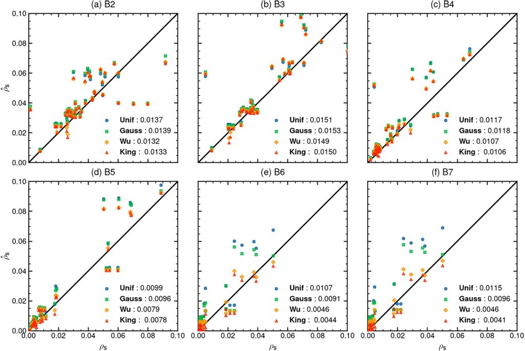
Although our MAJA processing pipeline is designed for land surfaces, in-situ reflectance measurements are most accurate over water, as on land, measurements are significantly affected by directional effects. We drew inspiration from the work of Wu et al. and used data from the Gloria database to compare different methods for correcting environmental effects applied to a large dataset of Sentinel-2 data. Some of the errors may come from the AOT estimate, which is measured by MAJA on land and extrapolated to coastal areas. These errors will be particularly noticeable in the blue and green bands (B2 and B3).

Starting from the red band (B4), and especially in the near-infrared (B6–B7), the improvement provided by our new PSF compared to the method currently used in MAJA (the Gaussian PSF) is particularly significant. Our model also performs slightly better than that of Wu et al. It is worth noting that our model will yield even greater improvements on land, where coupling effects—which were not taken into account by Wu et al.—are more pronounced.

A partir du rouge (B4), et surtout dans le proche infra-rouge (B6-B7), l’amélioration apportée par notre nouveau modèle par rapport à la méthode actuellement utilisée dans MAJA (la gaussienne) est particulièrement significative. Notre modèle fait aussi un peu mieux que celui de Wu et al. Rappelons que notre modèle apportera encore plus d’amélioration sur terre où les effets de couplage, non pris en compte par Wu et al, sont plus importants.

Conclusions and outlook

The new PSF model has therefore proven effective and our new correction will be implemented in MAJA. However, this presents a few challenges. The PSF now extends beyond 100 km; therefore, a convolution in the spatial domain would be too slow. The convolution must therefore be performed in the frequency domain to save time. However, this requires assuming that the PSF is constant within an image. However, we have seen that the PSF depends on the AOT, and variations in the AOT within the image cannot be taken into account with a fast Fourier Transform convolution..

Furthermore, the long range of these effects is problematic when the landscape beyond a certain limit is unknown. For example, very high-resolution data have a very narrow field of view. Pleiades has a field of view of 20 km, and CO3D has one of 7 kilometers. With these data, it will be very difficult to achieve a perfect correction, since we only know the landscape in a very small area. And even with wide-field images, such as Sentinel-2, the extensive spread of adjacency effects causes problems at the image edges. A commonly used solution is to extend the image by mirroring it at the edges, but this approximation is not valid if the landscape exhibits significant discontinuities.

Finally, our study did not take into account clouds, which are always heavily present in the atmosphere. For now, our correction method assumes that clouds and their shadows are “painted” onto the ground, whereas we would need to account for their 3D appearance. We have applied for a follow-up to this study as part of a new postdoc position, but our initial tests show that we would need to expand the cloud masks by several kilometers to ensure that the residual corrections for their environmental effects remain negligible.

References

• Wu Y., Knudby A., Pahlevan N., Lapen D., Zeng C. Sensor-generic adjacency-effect correction for remote sensing of coastal and inland waters, Remote Sens. Environ., 315 (2024), Article 114433, 10.1016/j.rse.2024.114433
• B.Bulgarelli, G.Zibordi, On the detectability of adjacency effects in ocean color remote sensing of mid-latitude coastal environments by SeaWiFS, MODIS-A, MERIS, OLCI, OLI and MSI, remote sensing environment, 2018, https://www.sciencedirect.com/science/article/pii/S0034425717305965
• Tanré, D., P. Y. Deschamps, P. Duhaut, and M. Herman (1987), Adjacency effect produced by the atmospheric scattering in thematic mapper data, J. Geophys. Res., 92(D10), 12000–12006, doi:10.1029/JD092iD10p12000.
• Vermote E., Tanre D., Deuze J., Herman M., Morcette J.J., Second simulation of the satellite signal in the solar spectrum, 6S: an overview, IEEE Trans. Geosci. Remote Sens., 35 (1997), pp. 675-686, 10.1109/36.581987
• Kévin Walcarius, Mustapha Moulana, Didier Ramon, Micaël Lassalle, Jérôme Colin, Olivier Hagolle, A revised model for atmospheric adjacency effect correction in optical satellite earth observation images, Remote Sensing of Environment, Volume 348, 2027, 115737, ISSN 0034-4257, https://doi.org/10.1016/j.rse.2026.115737.