Land cover maps quickly obtained using SPOT4 (Take5) data for the Sudmipy site
![]() =>
=> ![]() At CESBIO, we are developing land cover map production techniques, for high resolution image time series, similar to those which will soon be provided by Venµs and Sentinel-2. As soon as the SPOT4 (Take5) data were available over our study area (Sudmipy site in South West France), we decided to assess our processing chains on those data sets. The first results were quickly presented during Take5 user’s meeting which was held last October.
At CESBIO, we are developing land cover map production techniques, for high resolution image time series, similar to those which will soon be provided by Venµs and Sentinel-2. As soon as the SPOT4 (Take5) data were available over our study area (Sudmipy site in South West France), we decided to assess our processing chains on those data sets. The first results were quickly presented during Take5 user’s meeting which was held last October.
1. Experiments
In this post we describe the work carried out in order to produce these first land cover classifications with the SPOT4 (Take5) Sudmipy images (East and West areas) and we compare the results obtained over the common region to these two areas. Prior to the work presented here, we organized a field data collection campaign which was synchronous to the satellite acquisitions. These data are needed to train the classifier training and validate the classification. The field work was conducted in 3 study areas (figure 1) which were visited 6 times between February and September 2013, and corresponded to a total of 2000 agricultural plots. This allowed to monitor the cultural cycle of Winter crops, Summer crops and their irrigation attribute, grasslands, forests and bulit-up areas. The final nomenclature consists in 16 land cover classes. 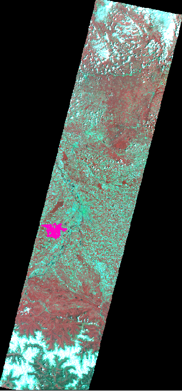
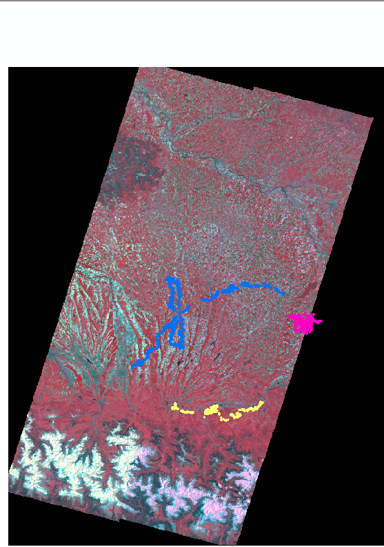 The goal was to assess the results of a classification using limited field data in terms of quantity but also in terms of spatial spread. We wanted also to check whether the East and West SPOT4 (Take5) tracks could be merged. To this end, we used the field data collected on the common area of the two tracks (in pink on the figure) and 5 level 2A images for each track acquired with a one day shift.
| OUEST | EST |
| 2013-02-162013-02-212013-03-032013-04-172013-06-06 | 2013-02-172013-02-222013-03-042013-04-132013-06-07 |
2. Results
The first results of supervised SVM classification (using the ORFEO Toolbox) can be considered as very ipromising, since they allow to obtain more than 90% of correctly classified pixels for both the East and the West tracks and since the continuity between the two swaths is excellent. Some confusions can be observed between bare soils or mineral surfaces and Summer crops, but these errors should be reduced by using LANDSAT 8 images acquired during the Summer, when Summer crops will develop.

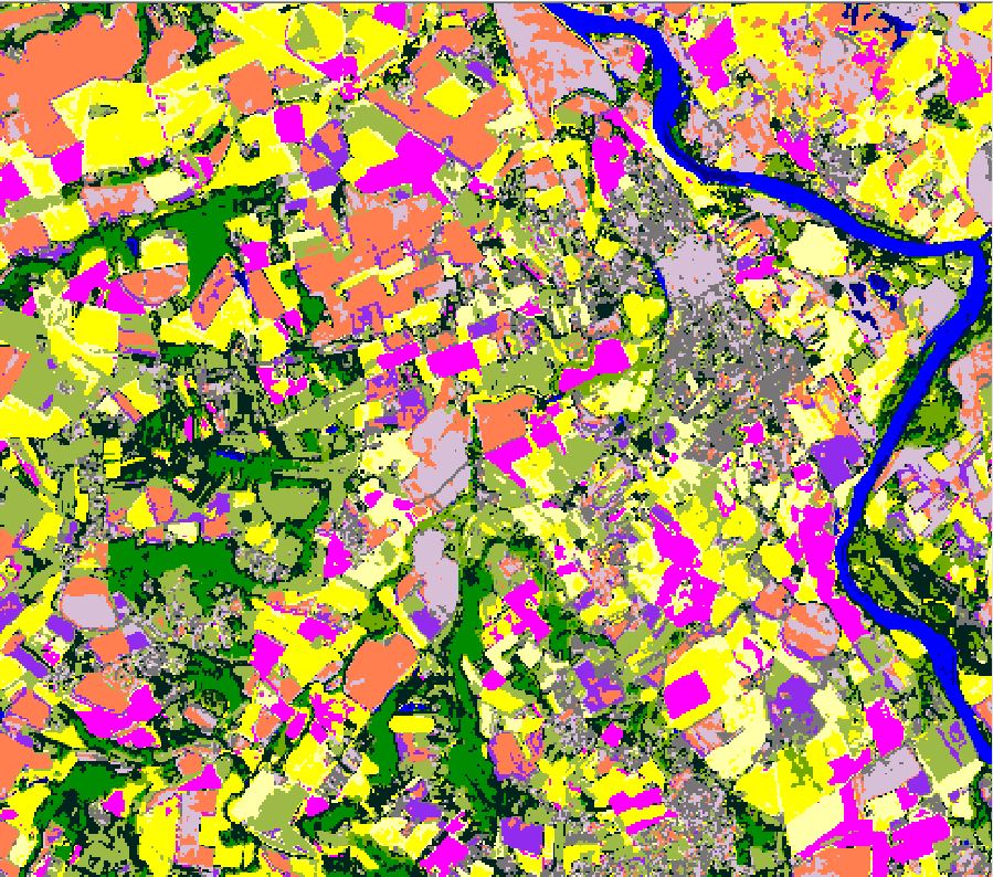
- Merging of the land cover maps obtained on the East and West Sudmipy tracks (the cloudy areas were cropped out). The comparison against the ground truth (the black dots on the map to the South-West of Toulouse) results in a kappa coefficient of 0.89 for the West and 0.92 on the East.
| West | EAST |
 | 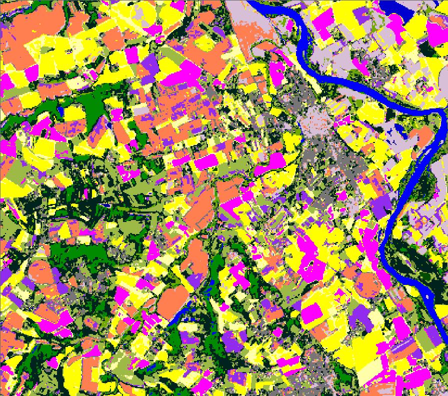 |
This zoom compares the results obtained on the common area of the two tracks (West to the left and East to the right). The two classifications were obtained independently, using the same method and the same training data, but with images acquired at different dates and with different viewing angles. The main errors are maize plots labeled as bare soil, which is not surprising, since this crop was just emerging when the last image was acquired. There are also confusions between wheat and barley, but even on the field, one has to be a specialist to tell them apart.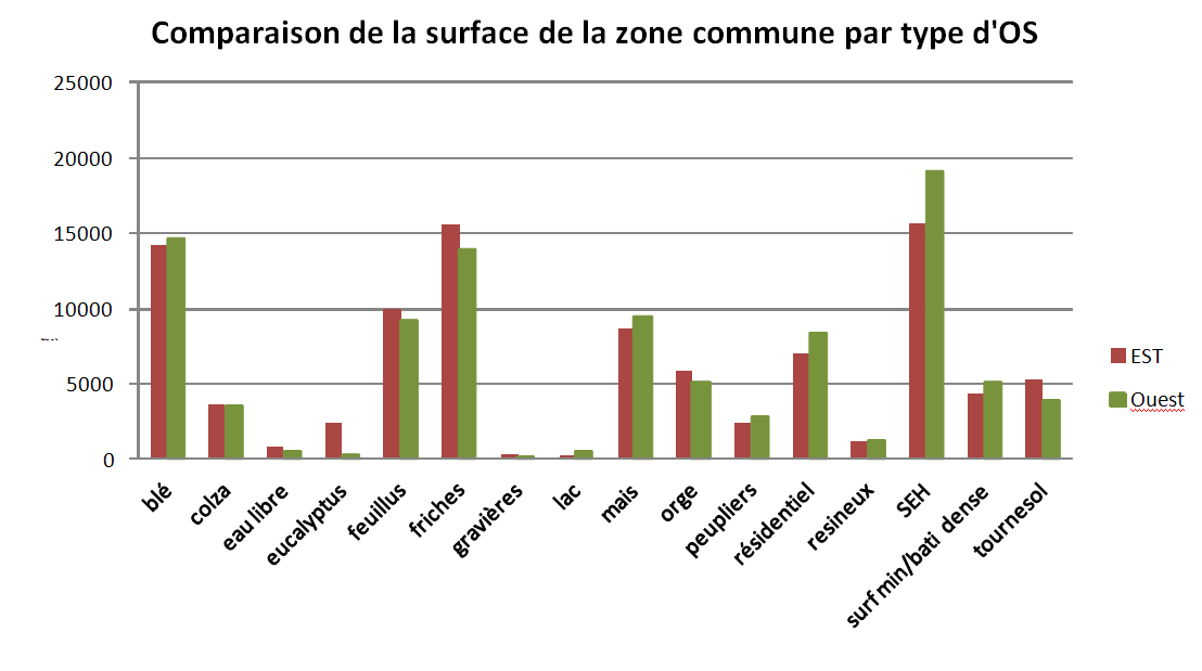
3. Feedback and retrospective
After performing these experiments, we were very satisfied with the operationnality of our tools. Given the data volume to be processed (about 10 GB of images) we could have expected very long computation times or a limitation in terms of memory limits of the software used (after all, we are just scientists in a lab!). You will not be surprised to know that our processing chains are based on Orfeo Toolbox. More precisely, the core of the chain uses the applications provided with OTB for supervised training and image classification. One just have to build a multi-channel image were each channel is a classification feature (reflectances, NDVI, etc.) and provide a vector data (a shapefile, for instance) containing the training (and validation) data. Then, a command line for the training (see the end of this post) and another one for the classification (idem) are enough.Computation times are very interesting: several minutes for the training and several tens of minutes for the classification. One big advantage of OTB applications is that they automatically use all the available processors automatically (our server has 24 cores, but any off the shelf PC has between 4 and 12 cores nowadays!).We are going to continue using these data, since we have other field data which are better spread over the area. This should allow us to obtain even better results. We will also use the Summer LANDSAT 8 images in order to avoid the above-mentioned errors on Summer crops.
4. Command line examples
We start by building a multi-channel image with the SPOT4 (Take5) data, not accounting for the cloud masks in this example :
otbcli_ConcatenateImages -il SPOT4_HRVIR_XS_20130217_N1_TUILE_CSudmipyE.TIFSPOT4_HRVIR_XS_20130222_N1_TUILE_CSudmipyE.TIFSPOT4_HRVIR_XS_20130304_N1_TUILE_CSudmipyE.TIFSPOT4_HRVIR_XS_20130413_N1_TUILE_CSudmipyE.TIFSPOT4_HRVIR_XS_20130607_N1_TUILE_CSudmipyE.TIF -outotbConcatImg_Spot4_Take5_5dat2013.tif
We compute the statistics of the images in order to normalize the features :
otbcli_ComputeImagesStatistics -il otbConcatImg_Spot4_Take5_5dat2013.tif -outEstimateImageStatistics_Take5_5dat2013.xml
We train a SVM with an RBF (Gaussian) kernel
:
otbcli_TrainSVMImagesClassifier -io.il otbConcatImg_Spot4_Take5_5dat2013.tif-io.vd DT2013_Take5_CNES_1002_Erod_Perm_Dissolve16cl.shp -sample.vfn "Class"-io.imstat EstimateImageStatistics_Take5_5dat2013.xml -svm.opt 1 -svm.k rbf-io.out svmModel_Take5Est_5dat2013_train6.svm
And Voilà !, we perform the classification:
otbcli_ImageSVMClassifier -in otbConcatImg_Spot4_Take5_5dat2013.tif -maskEmpriseTake5_CnesAll.tif -imstat EstimateImageStatistics_Take5_5dat2013.xml-svm svmModel_Take5Est_5dat2013_train_6.svm -out ClasSVMTake5_5dat_16cl_6.tif